Convolution

Building intuition for convolution from physical examples.

Convolution is an operation which takes two functions as input, and produces a single function output (much like addition or multiplication of functions). The method of combining these functions is defined as $(f\star g)(x)=\int_\Omega f(y)g(x-y)dy$ Where $x$, $y$ both range over all of $\Omega$. Here I will try and present convolution as a very convenient way of solving certain problems, and then abstracting from that; as a mathematical operation important in its own right.

Stones in Water

We will start our investigation by looking at some waves. Imagine you’re standing on the edge of a pond, and you throw a small stone in. The stone will cause a ripple to travel outwards across the surface. Bigger stones make bigger ripples, and smaller stones make smaller ripples, like so:

All three of the ripple patterns above share the same general shape, but differ only in their magnitude. How do we go about expressing this observation mathematically? First, let’s abstract a bit: if we look at the impacting stone as our input, and the resulting ripple as our output, we then have a process to model: $stone\to ripple$. We can express the dependence of the ripple’s size on the weight of the stone by saying that the output scales linearly with the input: $c\times \mathrm{stone}\to c\times \mathrm{ripple}$.

This property lets us see that there is some “special” stone we could study: that of unit weight. If we know the ripple caused by this stone, we can then find the ripple caused by any stone (lighter or heavier) by just scaling by the proper amount. If we think of this stone as appropriately “small” (technically, a point), then mathematically we can model it by an impulse. The wave caused by this unit weight pebble is called the impulse response, a relationship we can throw into symbols as follows: $\delta\to h$ where $\delta$ is the impulse and $h$ symbolizes the ripple. So far, by just knowing $h$ we are able to find the output which results from an input of any magnitude. What else can we do with it? Well; a lot it turns out. For one, so far we have been dropping our stones at the (mathematical) origin, but we intuitively expect the shape of our ripple to look the same no matter where we drop the rock. We can express this by saying that if we translate the impulse, we translate the response: $\delta(r-r_0)\to h(r-r_0)$.

What about if we drop two stones in at once, but at different locations? The wave caused by two stones is just the sum of the waves produced by each stone. In symbols, $\delta(r-r_0)+\delta(r-r_1)\to h(r-r_0)+h(r-r_1)$. Together with the scaling property we had from above; this lets us say our ripples are linear.

I’m going to replace the arrow with a function, $w$, so that instead of saying $\delta\to h$ we will say $w(\delta)=h$. Let’s say now that we have a handful of small pebbles of all different weights. We throw them into the water and they spread out, impacting at all different locations. How are we to model the complex ripple that will result? Well, upon impact, the surface just experiences a sum of stones $impact=\sum stones$, and each stone can be viewed as a scaled and translated version of our unit stone ($\delta$). This lets us say it a bit more precisely: $impact=\sum_i c_i\delta(r-r_i)$

Now, what does the wave that results look like? We can just apply our “wave operator”, w to the impact: $wave=w(impact)$, which we can phrase more mathematically by $wave=w\left(\sum_i c_i\delta(r-r_i)\right)$

We are now in a position to use our previous knowledge of the linearity of our “wave operator” to write this more explicitly: we know the wave of a sum is the sum of waves, and the wave of a scalar multiple is the scaled wave of the impulse, so we can go ahead and express this symbolically $wave=w\left(\sum_i c_i \delta(r-r_i)\right)=\sum_i c_i w(\delta(r-r_i))=\sum_i c_i h(r-r_i)$ Assuming we know the form of this function h then (the impulse response), we know the full form of our solution for the handful of pebbles:

This idea is at the heart of convolution as a solution technique - we found an initial configuration we understood well (a single impulse) and then when asked to solve a harder problem we attempted to write our new, more complex input as a sum of scaled and translated copies of this impulse we understood. Then we know the solution itself is just a sum of scaled copies of the response to that impulse!

However, the operation of convolution itself is an integral, and we sure don’t have anything like that showing up in our formulas yet. This motivating example is kind of like a “discrete convolution” - to arrive at the formula that begins this post we need to look at a different, more continuous example.

Blurry Cameras

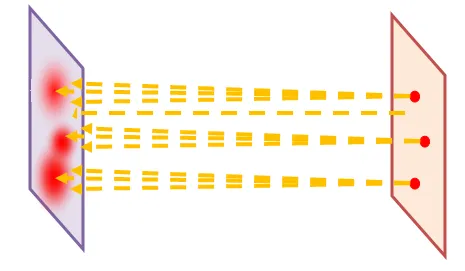
Instead of water waves, lets say we are going to take a picture. The setup is something like this: an object to be photographed, the camera lens system, and a piece of film.

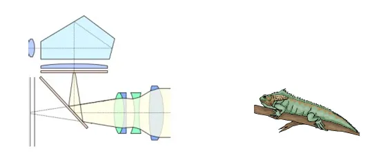
The goal of our camera is to take light from the original object and deposit it on the lens; so we can think of our camera as a function from object to film. If we call the object to be photographed the Source, the function to the image the Camera, and the film the Photograph, we can reduce this to a simpler schematic diagram.

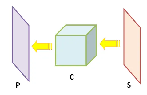
If we shine a bright light at the camera, we expect a bright image; if we shine a dim light, we expect a dim image. If we shine two lights, we expect two images. So, we can say that our camera function is linear, much like the waves. We can symbolize this relationship $P\stackrel{C}{\longleftarrow}S$ If our camera is in focus, we expect to see on the image exactly what what was around in the real world. That is, we expect a 1-1 correspondance between the source plane and the photograph.

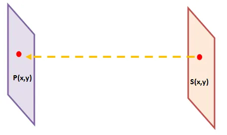
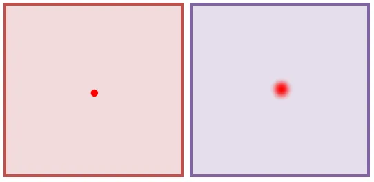
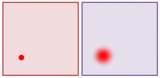
What if our camera is out of focus? We know from experience that this means what appears to be a single point in the source (think a star) is a smudged blob on our photo. Thus, we don’t have a 1-1 correspondence anymore, single source points spread their influence to multiple image points:

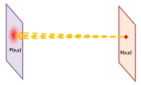
To make things easier to keep track of, we will let $h(x,y)$ stand for the blurry image of a star which was originally centered on the source screen (ie at $(0,0)$), after our crappy camera imaged it. Since this star is rather point-like, we will treat it as an impulse and say $\delta(x,y)\stackrel{C}{\longrightarrow}h(x,y)$

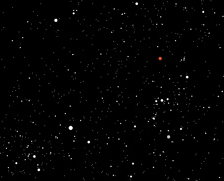
or $C[\delta(x,y)]=h(x,y)$. In exact analogy with our wave example, lets say now we take our camera and image the night sky. The source plane (the cosmos) contains a multitude of stars, each of a different brightness. What will our image look like? Well, just knowing how a unit impulse at the origin is imaged, we can figure it out! Viewing each star as a stretched and translated unit impulse; our image will be a collection of stretched and translated blurs. We can decompose the night sky into a sum of these modified impulses, and then distribute our imaging function over the sum, blurring each star individually and adding the results.

Symbolically say $Source=\sum Stars =\sum_i m_i \delta(x-x_i,y-y_i)$ Where $m_i$ is the brightness of each star, and $(x_i,y_i)$ is its spatial location.

If we want to determine what our photograph will look like, we can apply our function which represents the camera response to the source:

$$\begin{align}Image&=C[Source]\\ &=C\left[ \sum_i m_i \delta(x-x_i,y-y_i)\right]\\ &=\sum_i m_i C\left[\delta(x-x_i,y-y_i)\right]\\ &=\sum_i m_i h(x-x_i,y-y_i) \end{align}$$

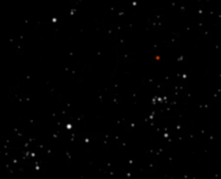
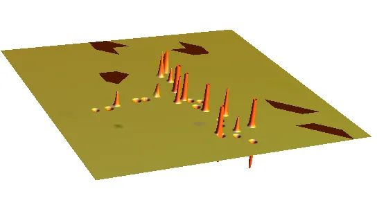
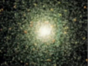
So far we have come up with two seemingly different problems; both which have a simple solution if we first understand how an “impulse” is propagated through them. Now lets take a picture of a portion of the sky with even more stars in it: for example, this small globular cluster which orbits our home galaxy:

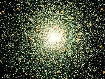
We can apply the exact same reasoning as above here: each star is like an impulse, so to see how each star will look on our final picture, we simply take that impulse, propagate it through the camera until it becomes our response function h, and then add all of them back together. The resulting blurry photo looks like this:

It’s time to make sure the mathematical formalism of this process really makes sense: at the location of each impulse (star), we apply our “blur” function which models our camera’s lack of focus. This blur function spreads the light out from this original point source to a more extended region. If our star is located on the source plane at point $(x_i, y_i)$, we need to make sure that our final image of the star is centered on that location as well. We defined our function $h(x,y)$ to be the blur caused by a unit impulse at the origin, so we need to slide this impulse to occur at our new point $(x_i, y_i)$ instead. This is what the term $h(x-x_i,y-y_i)$ says, it’s just a translated version of $h(x,y)$ centered at $(x_i,y_i)$ instead of $(0,0)$. Now if the stars original brightness was not simply $1$ but some other amount, we must scale the brightness of our blur accordingly. Thus the image of a star of brightness $m_i$ located at $(x_i, y_i)$ will be $m_i h(x-x_i,y-y_i)$.

So far, this has just been a more careful repetition of what we have done above. What we are going to do now seems to be a simple change of symbols, but will actually give us some profound insight into convolution itself. The number $m_i$ represents the brightness of our $i$th star, which is located at the point $(x_i, y_i)$ on the source plane. What this is really saying then is that the brightness of the source plane at location $(x_i, y_i)$ is given by $m_i$. That is, we can define a function on the source plane which gives us the brightness at each point. Lets call this function $m(u,v)$. Given a point $(u,v)$ of our source plane (the night sky), $m$ tells us what the brightness is there. Of course, in our star examples so far most points of the plane have a brightness of zero (black sky). But as we saw in the globular cluster, if we try to image a part of the sky with lots and lots of stars, some of them will seem to touch, and form extended areas of brightness.

In fact, in the limit lets say we find a point of the night sky where there are stars everywhere. There are no dark points, every line of sight ends in a star. Our brightness function $m$ would be nonzero everywhere, and every single point of the sky would have an impulse (star) located at it. Can we use what we have learned so far to figure out what our photograph of this area would look like? Sure we can! The only difference now is that we have a continuum of stars, instead of discrete points. But, at each location $(u,v)$ in the night sky, we have an impulse with brightness $m(u,v)$. We can represent this star by this brightness multiplied by an impulse function shifted to be located at $(u,v)$: $m(u,v)\delta(x-u,y-v)$ This single point source doesn’t propagate through our camera unchanged, however; it becomes blurred. This blur is still centered around the original location of the star however, and scaled for brightness by $m(u,v)$ so we can say the image of this particular star is $m(u,v)h(x-u,y-v)$.

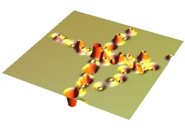
Just like in our discrete cases above, we now just need to sum up the images of each star to get the final image. This sum needs to be taken over each $(u,v)$ which has nonzero brightness, which in the present case is all of them! We will need to perform a continuous sum then, over each position $(u,v)$. $\int_{\mathbb{R}^2}m(u,v)h(x-u,y-v)dudv$ This last equation just says the image of our continuous field of stars is the blurred image of each star individually, all added back together. However, this also happens to be a realization of the formula for convolution presented at the top of this post! The resulting image of our star field is just the convolution of our brightness field with the blurred image of a unit star at the origin! $photo=m(x,y)\star h(x,y)$ How about the image of a lizard? Well, we were able to treat a continuous field of stars successfully by modeling it via a continuous “brightness” field. What if we just view our lizard as a continuous field of brightness/color? With the stars it was intuitive to say that each point was in reality an “impulse,” which was the crux of our argument. Does the same thing carry over here? Is the image of a lizard really nothing more than a weighted collection of impulses? Let’s think for a second about a television set displaying our lizard on it’s screen. If you get really close to this image, you’ll notice that its actually made out of teeny tiny pixels, its nothing more than a collection of tiny impulses! If we shrink these pixels to zero size (as an ideal impulse is), then it seems we can really say that a lizard’s image is nothing more than a collection of infinitly small pixels, or impulses! Since we already know how our camera responds to a unit impulse, all we have to do to model the photo of our lizard with the blurry camera is to take this response, scale it by the brightness at each location, and add them all up.

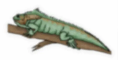
(Its probably time for a new camera!)

The blurry image is then just the convolution of our original image of the lizard (the brightness field), and the response of the camera to a single impulse.

Back to Water Waves

Alright then, back to the water waves. What if we threw a larger object into the pond? Instead of having a discrete set of impulses to start the water vibrating, we have a continuous field of applied pressure $p(x,y)$. Just like with the image of the lizard, we can look at this continuous field as simply being a bunch of scaled impulses smushed up next to each other. To find the wave caused by this, we just need to find the wave caused by a single impulse, translate it, scale it, and add them all up

$wave=\int_{\Omega}p(u,v)h(x-u,y-v)dudv$

Again, we recognize this as a convolution of the wave caused by a single impulse and the pressure field of the extended object:

$wave = p(x,y)\star h(x,y)$

These two examples give us a bit of a feel for what convolution is. If we know how a certain system reacts to a simple impulse, we can figure out how that system reacts to anything, by first breaking it down into impulses, sending each through individually, and adding them up at the end. When we add them all up, we have to make sure to shift all the functions appropriately and scale them (so it matches up with the input) and taking care of this turns our sum into a convolution integral. Convolution is just the continuous analog of the problem solving strategy “break it down into small parts, solve those, and put em back together at the end”.

This is of course not just useful for waves (water, or electromagnetic, as we’ve seen so far) but to any system where an input can be broken down linearly into a continnuum of tiny impulses. Then the overal behavior is just the continuum of simple impluse responses. We explore one final example below.

Heat

Consider for a moment a metal rod which we have heated in some way. If we let it sit out, it will obviously cool down, but how do we express this quantitatively? Via a partial differential equation known aptly as the “heat equation”, given the initial temperature of our rod (as a function of position), we can solve for its temperature at all future times.

$\partial_t u = \partial_{xx}u\hspace{1cm} u(x,0)=f(x)$

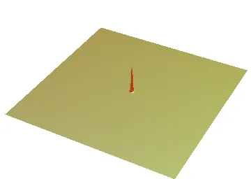
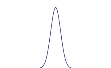
For a general initial temperature distribution this may be a hard thing to do. So let’s see if we can stick to the reasoning that’s proved fruitful so far, and consider the effect one “impulse” of heat has on our rod. The mathematical model for this sets the initial condition to $\delta(x)$, and the solution to this problem is called the “fundamental solution”, and can be visualized as follows:

In this image, the red represents “hot” and the blue “cold”. At t=0, we apply an impulse of heat to our rod (think of touching a soldering iron to it), and as time progresses that heat spreads out and evens out, as we would expect it to. We can alternatively choose to plot the heat distribution in a “standard” graph:

Where the vertical dimension gives the temperature at position x. Solving the heat equation analytically for this particular initial condition, we can arrive at a closed form of this fundamental solution

$F(x,t)=\frac{1}{2\sqrt{\pi t}}e^{-\frac{x^2}{4t}}$

The most important part however is not the form of this solution, but rather the form of the problem: the transformation of our initial impulse into a different function:

$\delta(x)\mapsto F(x,t)$

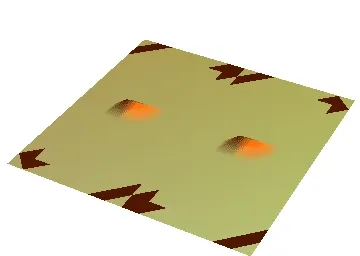
If we had decided to place the soldering iron at a different location than the origin, we would expect the same heat distribution to result, and so this process is translation invariant. Had we placed two soldering irons, we would expect the result to be the sum of two dispersing heat waves, and if we had placed a hotter iron, we would expect a hotter rod; the heat equation is linear and translation invariant.
In abstract-land, this problem is identical to both of the above. We have some sort of a correspondence between an impulse and a function, and we can write this correspondence in a linear, translation-invariant manner. Thus, we expect that if we heat the bar via some continuous distribution instead of an impulse, we can find the final solution to our problem by convoluting the initial temperature with the impulse response. As an example lets say we heat the bar to the right of the origin, and cool it to the left so that the initial temperature distribution looks something like this:

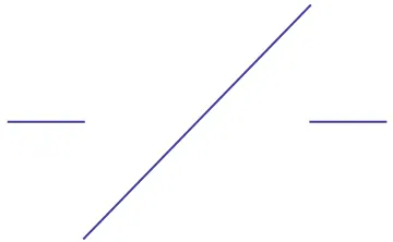
Or, in symbols its a piecewise function with $f(x)=0$ for $|x|>3$ and $f(x)=x$ for $|x|<3$. To solve for the temperature distribution caused by this initial condition, we will view f as being composed of a bunch of mini impulses, right next to eachother. Feeding each impulse through the heat equation will give us a shifted and translated version of our fundamental solution, and adding them all back together will give us the answer we seek. This is of course, just the convolution of the initial condition and the fundamental solution:

$$\begin{align} u(x,t)&=f(x)\star F(x,t)\\ &=\int_{\mathbb{R}}f(y)F(x-y,t) dy \end{align}$$

Since our initial condition is only nonzero over the finite range [-3,3], we can simplify this integral as

$$\begin{align}u(x,t)&=\int_{-3}^3 f(y)F(x-y,t)dt\\ &=\int_{-3}^3y F(x-y,t)dt\\ &=\int_{-3}^3 \frac{y}{2\sqrt{\pi t}}e^{-\frac{(x-y)^2}{4t}}dy \end{align}$$

While not computable using the methods of a calculus course, this integral is easily evaluated in terms of the Error function $\mathrm{erf}(x)=\frac{2}{\sqrt{\pi}}\int_0^x e^{-u^2}du$ by a computer algebra system:

$$u(x,t)=\frac{1}{2} x \left(\text{erf}\left(\frac{x+3}{2 \sqrt{t}}\right)-\text{erf}\left(\frac{x-3}{2 \sqrt{t}}\right)\right)+\frac{\sqrt{t} \left(e^{-\frac{(x+3)^2}{4 t}}-e^{-\frac{(x-3)^2}{4 t}}\right)}{\sqrt{\pi }}$$

This is the explicit solution to the heat equation for our initial condition. Pretty amazing! Plotting this as a temperature distribution and a graph

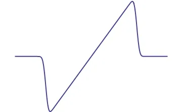
We can see qualitatively that the temperature distribution tends to “smooth out” as time progresses, much as we would expect. This example provides some good mathematical justification for the use of convolution: in addition to it being intuitively simpler to break a problem into impulses and then just re-combine them, it’s hard to see how to even come up with an analytic expression as complicated as the solution here if we had not first solved for the fundamental solution, and then gone used convolution formally to compute the desired answer.