Exponential Functions and the Number e

Starting from repeated multiplication and arriving at a universal constant.

The family of exponential functions (things of the form $a^x$ ) are ubiquitous in mathematics, physics and engineering. Due to the relatively simple set of rules for manipulating such expressions, once learned they can be used almost without thinking, and often the meaning behind them is lost. Thus, instead of a rigorous approach, I will try to provide some bits of intuition, specifically focused on what makes e such a “special” number.

Integer Exponents

Exponentials first arise out of a need for a shorthand for multiplication (much like multiplication itself can be seen as a generalization of a shorthand for addition). Lets say we have a number $a$ which we’ve multiplied together a bunch of times to get $b=aaaaaa$. Since there are 6 $a$‘s in this expression, we decide to write it $b=a^6$. The rules of exponents learned in high school are just a consequence of this notational choice. To see this, consider the number $a^4$ and $a^2$. Since these are just short hand expressions for the product of four $a$‘s and two $a$‘s respectively, it is easy to see what the shorthand of their product should be:

$a^4\cdot a^2= (a\cdot a\cdot a\cdot a)(a\cdot a)=a\cdot a\cdot a \cdot a\cdot a\cdot a=a^6=a^{4+2}$

And in general, multiplying a product of $m$ successive $a$‘s and a product of $n$ successive $a$‘s simply gives a product of $m+n$ successive $a$‘s. In our shorthand then; $a^m\cdot a^n=(a\cdot a\cdot a \cdots a)(a\cdot a \cdot a\cdots a)=a\cdots a=a^{m+n}$

Which is nothing other than the standard rule for exponents. Now say that you have a number $b$ which happens to be a product of three $a$‘s, that is $b=a^3$. Is there a “nice” way to talk about the product of $b$ with itself five times? If each $b$ is composed of three $a$‘s and we have five $b$‘s multiplied in succession, then another way to phrase this is simply that we have 15 $a$‘s being multiplied together. In the exponential shorthand;

$(a^3)^5=a^3\cdot a^3\cdot a^3\cdot a^3\cdot a^3= (a\cdot a\cdot a)\cdot(a\cdot a\cdot a)\cdot(a\cdot a\cdot a)\cdot(a\cdot a\cdot a)\cdot(a\cdot a\cdot a)$ $a\cdot a\cdot a\cdot a\cdot a\cdot a\cdot a\cdot a\cdot a\cdot a\cdot a\cdot a\cdot a\cdot a\cdot a =a^{15}=a^{3\cdot 5}$

This also extends arbitrarily; $(a^m)^n$ says to take the number $a$ and multiply it together $m$ times, and then take that and multiply it by itself $n$ times. Obviously $n$ copies of a set of $m$ objects placed side by side is just a list of things of length $mn$. This is then written in our exponential shorthand as $(a^m)^n=a^{mn}$.

This idea of using exponents as a short hand for repeated multiplication has turned out to be quite useful, so lets see how it extends. As of now our preliminary definition is restricted to positive integer exponents (because it only makes sense to multiply things together an integer number of times). What about negative integers? If positive integer exponents give us a short hand for repeated multiplication, could it be possible to define negative integer exponents to be a short hand for repeated division? Much like $a^5$ means “multiply $a$ by itself five times”, then $a^{-5}$ would signify dividing by $a$ five times. This turns out to work well with the exponent rule above: say you multiply by $a$ five times and then divide by $a$ three times. This is obviously equivalent to only having multiplied by $a$ twice, so in effect we would like it to be true that $a^5a^{-3}=a^2$. But by our rule for dealing with this short hand, we already know that $a^5a^{-3}=a^{5-3}$, so it all checks out! This gives some confidence that there is no real issue with extending the exponential short hand to both positive and negative integers, allowing it to represent both repeated multiplication and division.

This also allows us to assign meaning to the idea of “a product of no $a$‘s at all”. Since in our shorthand this would be represented by $a^0$, as of yet we have not explicitly given it a meaning (we have only defined what it means to raise $a$ to the power of a positive or negative integer). It might seem that this is a case we should just ignore, for when are we ever going to need a product of zero $a$‘s? However, if we expect to take this notation seriously then the notion of $a^0$ is forced upon us naturally: it is the symbol we would use to represent first multipliying by $a$ and then dividing by $a$ ( as this would be written $a^1a^{-1}=a^0$). In fact, it is the symbol which represents multiplying $a$ by itself $n$ times and then going on to divide by $n$ copies of $a$ for any $n$. Since $a/a=1$, it follows that to be consistent we must say that $a^0$ is just another symbol representing the multiplicative identity, which gives us the nice interpretation “multiplying something by a product of no $a$‘s dosent do anything at all”:, or in symbols $a^0=1$.

Thus, when taking integers as input; exponentials can be thought of as just a way to save paper (long strings of $a$‘s aren’t very enlightening to write down). Theres no real new information here, and the rules of exponents are just a way of codifying the nature of repeated multiplication.

Rational Exponents

Given our current view of exponentials as just a shorthand for multiplication; it might seem silly to try and stick a meaning to something like $a^{\pi}$. However a lot of interesting mathematics falls out of trying to extend things that appear useful and simple. Its good to keep in mind that right now, the above expression doesn’t make any sense. Until we give it a meaning, its just a collection of symbols. To avoid jumping the gun, we will first try to define a simpler concept: a number raised to a fractional power. In fact, it would probably be easiest to start with an example: let’s try and give meaning to the expression $a^{1/2}$. We would like everything we do in extending the exponential notation to be compatible with the case where it is intuitive (integer exponents), so in particular we would like $a^{1/2}a^{1/2}=a^{1/2+1/2}=a^1=a$. That is, to be consistent we need $a^{1/2}$ to be the number that when multiplied by itself gives $a$. This number already has a name; the square root of $a$. Thus we have a guess at a possible extension: $a^{1/2}=\sqrt{a}$.

What about sticking other fractions in exponent? If we say that $r$ is some general fraction, then we can write $r=p/q$ for two integers $p$,$q$. Because we want our extension to be consistent with the rules from before; we can write $a^r=a^{p/q}=(a^{1/q})^p=a^{1/q}a^{1/q}\cdots a^{1/q}$ Thus the number can be identified with the $q$th root of $a$. This gives us a nice way to define all rational exponents. Any rational exponent of $a$ can be looked at as being $p$ copies of the $q$th root of $a$ multiplied together, for some $p$,$q$. This lets us look at an expression like $a^{14/3}$ and know that it simply means to take the cube root of $a$, and multiply it by itself 14 times.

Without going into any depth (this is only supposed to help provide intuition, after all), we have a pretty good grasp on the exponential function. Positive integer exponents are just a shorthand for repeated multiplication. Negative integer exponents are just repeated division. Exponents of the form $1/n$ are just an alternative way of writing the $n$th root. By combining these simple cases, we can find the value of any rational exponent.

Real Exponents

What about the irrationals, though? The real line is chalk full of ‘em; so aren’t we missing a lot here? Well, yes and no. The good thing about the rationals are they are everywhere…pick any little piece of the real line, no matter how small you’d like, and there’ll be a rational number in it (actually, there’ll be infinitely many of them). So from an intuitive standpoint, it’s probably easiest to think of the exponential as having a nice interpretation on the rationals, and then just being forced to take the correct values on the irrationals to “fill in the gaps”. This can be made more precise by noting that $\mathbb{R}$ is separable (it has $\mathbb{Q}$ as a countable dense subset ) and so the values of any continuous function over $\mathbb{R}$ are totally determined by the values it takes on $\mathbb{Q}$ (which, in our case, have been completely described). Thus, the value of something like $a^\pi$ is forced on us because we know the values of a raised to the power of all rationals nearby $\pi$, and this is as precise as we will need.

The Laws of Exponents: Geometrically

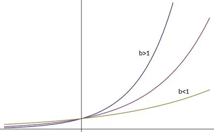
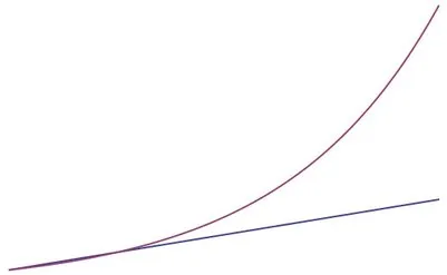
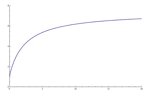
Once we begin thinking about real number exponents, we can think of the exponential in terms of its graph, and try to reason about it from that perspective. What does the graph of an exponential function look like? Well, generically they look like this:

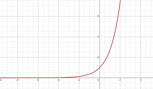
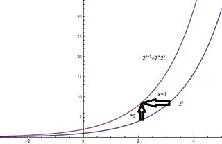
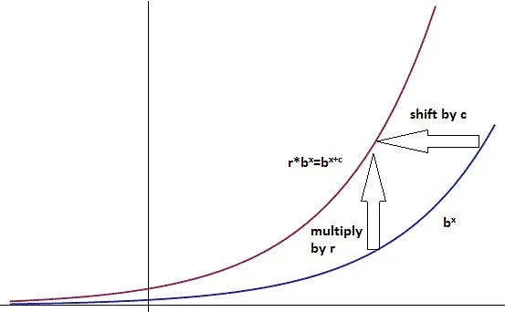
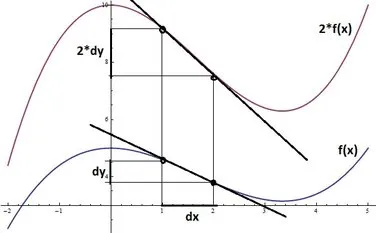
But this isn’t just any old upward moving squiggle with a horizontal asymptote to the left: the properties of exponentials we discovered above force the exponential graph to have some very special properties. For instance, how can we interpret the rule $a^na^m=a^{n+m}$ geometrically? As an example, lets take a=2. What happens if we multiply each point on the graph by two? This would amount to a vertical stretching of the graph, moving each point twice as far from the x axis as it originally was. Algebraically, this new function is $2\times 2^x$, which by the laws of exponents can be rewritten as $2^{x+1}$. Quick recap: our original function was $2^x$ , and we doubled it to get $2 2^x=2^{x+1}$. However this is simply the original function shifted to the left by 1. Thus stretching vertically by a factor of 2 produces the same result as shifting the graph to the left by 1. This is shown below.

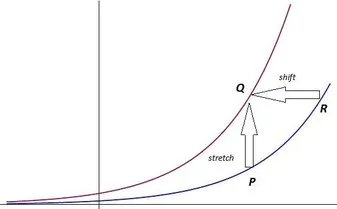
This is a special property of exponentials; their self-similarity. Stretching one vertically is equivalent to translating it horizontally instead. Lets see to what extent this is true. Lets pick some arbitrary exponential $a^x$, and some point $P$ on its graph (this is the blue graph in the figure below). If we let $r$ denote the x-coordinate of $P$, the y-coordinate of $p$ is simply $a^r$. Now lets stretch this entire graph vertically by a factor $k$. The new graph, $ka^x$ is purple in the below figure. If $k$ is a positive number, then we can find some number $c$ such that $k=a^c$ . This allows us to re-express $ka^x$ as $a^{c}a^x$, or equivalently $a^{x+c}$. Thus we have the relation $k a^x=a^{x+c}$ If we let $Q$ denote the point on which is the stretched image of $P$, this gives us a second way of getting to $Q$ from the original graph: we can start at the point $r+c$ on the x axis, and move vertically to a point $R$ on $a^x$. Shifting this point horizontally $c$ units to the left gives the point $Q$, which is a translated image of $R$.

The geometric interpretation of the first “law” of exponents can then be stated as follows: if $f(x)$ is some exponential function, then a stretch of the form $kf(x)$ is equivalent to a translation of the form $f(x+c)$. This is a property that can be observed on a graphing calculator or with a computer algebra system: as you zoom in on an exponential curve, provided you scale the axes right, it looks the same at any size. This self-similarity is the basis of the “memoryless” property of the exponential distribution often quoted in statistics, and will help us understand exponential derivatives in a bit.

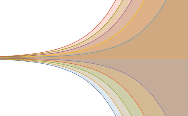
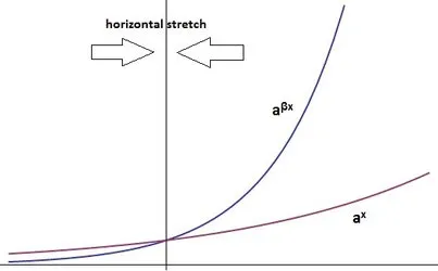
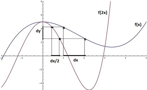
We have taken a look at what happens when we stretch an exponential vertically, but what about if we stretch it horizontally? A horizontal stretch is a stretch of the x-axis, and so we can accomplish it algebraically by replacing $x$ with $bx$ in our formula. For $b<1$, this corresponds to an expansion, and $b>1$ is a contraction, or squishing of the graph about the x-axis origin. This is illustrated below.

From the above pictures, it appears reasonable to assume that a horizontal stretch (either compression or expansion) produces yet another exponential function. To take a concrete example, lets go back to our old friend $2^x$. This graph can be horizontally compressed by replacing $x$ with $2x$, giving $2^{2x}$. These two exponentials are shown below.

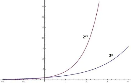
Because throughout our extension of exponentiation from the integers to all real numbers we forced the identity $(a^m)^n=a^{mn}$ to hold, we can use this to re-express our compressed exponential in a more insightful way. In terms of the example, $2^{2x}=(2^2)^x=4^x$

And so a horizontal compression is equivalent to a change of the exponential base. Given an exponential $a^x$, the effect of a horizontal stretch $x\mapsto b x$ is really just a change of base. If we let $c$ stand for the value $a^b$, then a stretch of factor $b$ is equivalent to the change $a^x\to c^x$.

Thus we have two ways to look at the rules for manipulating exponents: either we can view them algebraically as simply facts about what must be true for integer exponents to make intuitive sense, or we can view them as statements about how vertical and horizontal stretches of an exponential graph really end up resulting in translations or changes of basis. The ability to get from one exponential to another by two quite different means is a pretty useful property for intuition: in fact, these properties allow you to look at any exponential whatsoever as just a squished copy of some other exponential. To see this, we are going to need to know a little about undoing exponentials; so i’ll pick up on this train of thought again in a bit.

Logarithms and Rewriting Exponentials

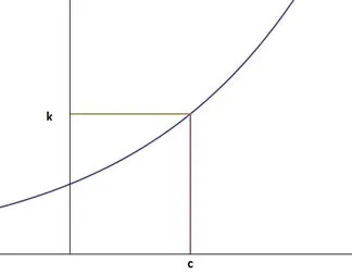
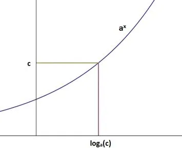
In the last section at one point, we had a number $k$, and we claimed that it was possible to rewrite this as $a^c$ for some $c$. Why can we do this? A quick picture will help here; plotted below is an arbritrary exponential curve, with some number $k$ selected along the y-axis. Looking at the corresponding x value (call it $c$) we notice that for this particular choice, $k=a^c$ as required. So long as $k>0$, this argument applies in general; its easy to see that there will always be some corresponding x value.

Finding such a $c$ for a given $k$ is an inverse problem (given the output of the function, $k$, find an input $c$ such that $f(c)=k$), and thus we are in need of an inverse function for the exponential. Since all exponentials are bijective functions, they are invertible, and we can actually do this. Geometrically an inverse function is simply the reflection of the original function over the line $y=x$; a graph of both an exponential and its inverse is shown below.

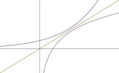
To not wander too far astray, we won’t spend too much time worrying about the inverse function, hopefully the above illustration is enough to provide some feeling that it exists (the proof is simple; just verify the injectivity and surjectivity of the exponential as a map ). Now that we know there is one, to be able to discuss it precisely we need a good notation for it. If we have the exponential $a^x$, then we will denote its inverse by $\log_a(x)$, and call such a function the logarithm with base $a$. This function is defined exactly like the first picture in this section; if $b$ and $c$ are numbers such that $a^b=c$, then $b=\log_a(c)$. Pictorally;

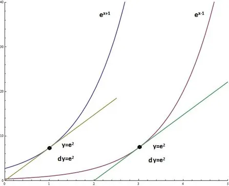
Ok, we’ve covered enough stuff now to discuss how the self-similarity properties of exponentials allow us great freedom in how we write them (and interpret them). Lets say for some reason or another, you’ve found a particular exponential function that you really like, call it $a^x$. You’re working on some problem and another exponential shows up; something that superficially bears no resemblance to your favorite member, we’ll write this guy $b^{x+c}$. There might be good physical reason that this exponential has the form it does, but no matter; whatever the source of this particular exponential there is a way to interpret it as simply a stretched copy of your $a^x$. To see this, lets first consider the form of the exponential you were given. It is the simple exponential $b^x$ , after a horizontal shift of $c$ units to the left. We know from previously that a horizontal shift is really just a vertical stretch, and so we can think of as being $rb^x$, for a vertical stretch factor $r$ (this stretch factor can easily be seen to equal $b^c$).

Now what about the remaining exponential? It is still the wrong base; so we need a way of viewing $b^x$ as some stretched copy of $a^x$. We saw previously that change of base is really just a horizontal stretching, so we know that theres a way to write $b^x$ in the form $a^{\beta x}$, for some horizontal stretch of magnitude $\beta$. The value of $\beta$ satisfying this can be found using the exponent laws: we want to satisfy the equation $b^x=a^{\beta x}$, so we need $b=a^\beta$. If we now view $\beta$ as a variable in the exponential function with base $a$, we have a situation that has already been discussed: we know the y-coordinate of some point on the exponential curve , and we want to find the x coordinate. This can be accomplished using the inverse function; giving us our answer $\beta=\log_a b$

Thus we have the formula $b^{x+c}=ra^{\beta x}$ and the values of $r$ and $\beta$ which satisfy it, allowing us to view our arbitrary exponential as really just $a^x$, stretched horizontally by $\beta$ and vertically by $r$. Below is an animation of how the two stretches in unison actually achieve this:

Exponentials and Growth

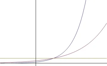
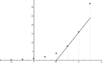
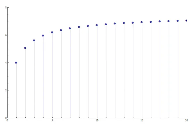
Our first introduction to exponentials was their discrete nature, as an extension of multiplication. However this is not the only situation in which they arise, heck it’s not even what makes them most useful. Passing from an algebraic shorthand to their continuous case left us with a set of functions over with some pretty cool properties. One of the most useful interpretations of exponentials is that of growth, they are the natural choice of a mathematical model for a kind of growth which depends on how much “stuff” is already present. To see this, we will first take a step back and consider the nature of growing things in general. The simplest kind of growth is linear growth: say each day you are given a dollar from your friend. After 5 days, you will have 5 dollars, after x days, you will have x dollars. Your riches grow linearly with time. The amount of money you will make tomorrow doesn’t depend on how much money you have today; regardless of if you are broke or a millionaire, you will make one dollar tomorrow. Now lets consider a different scenario: someone gives you a dollar, and you invest it in some ridiculous company which promises to double your total investment each day. So, the next day they give you a dollar, doubling your current amount. The second day however, they give you 2 dollars, so you now have a total of 4. The following day they double that, giving you 4 so that you have 8. Continuing this process, you see that your dollar amounts each day form the list {1,2,4,8,16,32,64,…}, which is nothing other than the table of values for 2x. In this model of growth, the amount you earn tomorrow depends on how much you have today: if you have 1 dollar you will make a dollar, if you got a million, you’ll make a million. The striking difference between these two modes of growth can be seen below

Looking at exponentials as a form of growth allows a nice physical interpretation of the “vertical stretch = horizontal shift” we talked about: say you’re that lucky investor whose total investment is doubled each day. If you start on day 0 with 1 dollar, your income is modeled by $2^x$. But what if you started by investing 8 dollars? your income on day 2 would be 16 dollars, making your total 32, your total the next day would be 64, then 128, and so on. In fact, each day you will be making as much money as the guy who invested a single dollar does 3 days later. Your income is simply his income shifted by 3 days. Thus investing 8 dollars to begin with (stretching the income function by a factor of 8 vertically) is the same thing as just having invested a single dollar 3 days earlier (shifting the income function horizontally by a factor of 3).

In fact, any growth process where your amount of growth is proportional to how much you have at the moment is a form of exponential growth. Tripling your total amount each day is the exponential $3^x$, quadrupling amounts to $4^x$. Heck even multiplying your total by $12.3456$ (or any other random number) each day is modeled by the function $(12.3456)^x$. These examples have all been of the discrete case, but the same intuition carries over to the continuous case: if you have a growth rate which is proportional to the amount of stuff you have, the growth will be exponential. We can formulate this more precisely in the language of differential calculus: let $y(t)$ be a function which for each time outputs an “amount”. At a given time $t^\ast$, the rate at which y is growing is its derivative, $y'(t^\ast)$. To say that the growth rate is proportional to the amount of stuff you have, is to say that the derivative is proportional to the function’s value at that point $y'(t)=ry(t)$ The functions $y(t)$ which satisfy this are the exponentials that we have been discussing all along (I wont bother deriving why…the usual proof involves knowing that a certain integral comes out to be the natural logarithm; a fact that here doesn’t help much with intuition). Hopefully the analogy of this differential equation with the discrete case is at least suggestive that both should follow the same general trend.

The Special Number $e$

It seems you can almost not hear of or work with exponentials without encountering that seemingly random irrational number, $2.71828182....=e$. It’s one of those things that is mystifying the first few times you see it, but it comes up so often that before long it is second nature to use. However, during the learning process (at least in my experience) using $e$ for years never really gave a good sense of exactly what made it special. $e$ is singled out for multiple different reasons, which is probably why it’s hard to see any underlying theme when learning to use it.

First of all, you may ask, why would there even be any “special” base for the exponential? What has been discussed so far has been done in full generality; with $a$ serving as a placeholder for any base you could want. In this sense, it seems that all possible exponentials are created equal. Sure, we can pick some $a$ that we like and write all exponentials as just stretched versions of it; and this might be a very convenient thing to do (computationally you would only ever have to worry about one exponential function, and just feed it different arguments), but how could there be a natural way to select such a base? My goal here is to convince you that there is a natural choice, that the choice is $e$, and that the various ways of defining this number actually share a common theme.

Lets start back with the idea of exponentials representing growth: out of all discrete growth rates, the one singled out as “special” is the unit growth rate; or an increase of 100% of your amount each day. This is our friend $2^x$ from before, but lets see why. As we argued before, discrete exponential growth is a process where the gain over each unit of time is proportional to the current amount. Say the current value on a given day is $P$. Since the gain on the next timestep is proportional to $P$, we can write $gain=rP$ for some proportionality constant $r$. The amount you have at the end of that next time step is then the previous amount plus the gain: $P+rP$. We can factor the current amount out of this equation, giving $(1+r)P$. This gives the total amount at a given time in terms of the amount at the previous time. Letting $P$ vary with $n$; $P(n+1)=(1+r)P(n)$ Solving this recurrence relation gives $P(n)=(1+r)^nP(0)$ Which gives the amount at all future times in terms of the initial amount in terms of a stretched exponential with base $1+rate$. Setting the rate of growth to unity (that is, making the proportionality above an equality), gives us the equation $P(n)=P(0)(1+1)^n=A2^n$, which justifies the fact that discrete growth at a unit rate is modeled by $2^x$.

The natural question is then, can we extend this notion of “unit growth” in some way to the continuous case? That is, is there any continuous exponential which we can say grows at unit rate? From our look at the discrete case we have learned two properties of unit growth which can be used to characterize it: namely that the proportionality constant between growth and current value is 1, or that at any instant in time the rate of growth is equal to the current value. How would we phrase these requirements in the continuous case? We saw before that if the growth rate is proportional to the value, we have the condition $y'=ry$. Setting $r$ to unity in this equation gives us a differential equation for unit continuous growth: $y'(t)=y(t)$ The solution to this equation will then be the function which we can say grows with unit speed. Since we know by the equation’s form that it is an exponential; all we must do is find which base satisfies it. For lack of a numerical value, lets call the base $e$. Stepping back from our current question about growth rates and looking at the equation itself, it turns out we have run into another quite interesting problem. This equation selects functions $y$ which are their own derivative. That is, unit growth is equivalent to the condition that the differential operator have no effect on the function. Without considering our reasoning that got us to this equation, it may seem unlikley that it has a solution at all: after all, if it does that means that there must be a function out there which remains invariant under differentiation. However phrased in terms of growth rates, we know there are exponentials with growth rate less than 1, and those of growth rate greater than 1; so it makes intuitive sense that there should be some exponential in between, with growth rate of exactly 1. Thus for now, we are going to assume this equation is solvable, and see what we can learn about the qualities of its solutions.

Looking at the differential equation, we see that it is first order in $t$. Without initial conditions, this implies that there is a 1-parameter family of solutions to this equation, which we will index by $a$ and call them $y_a(t)$. Also, this equation only mentions the derivative at t and the y-coordinate at t, never the actual t value at which they occur. Because of this, we can see that given a particular solution of this equation, say $y(t)$ then $y(t-a)$ is also a solution (use the chain rule).

This tells us that the solutions to this equation are all related to each other by the translation of one basic solution to the left or right. Since we additionally know the solution must be exponential, we can use our geometric interpretation of the laws of exponents to notice that shifts to the left or right are equivalent to vertical stretches. This lets us write our one parameter family of solutions as $y_a(t)=ae^t$

How do we go about finding the value of this base $e$? Lets look quickly back to the discrete case for some help. Considering our unit discrete growth function of $2^n$ , look at the discrete analog of the derivative at a point, the slope of the secant line defined there. At a given $n$, we have $\frac{\Delta(2^n)}{\Delta x}=\frac{2^{n+1}-2^n}{(n+1)-n}=2^{n+1}-2^n=2^n$

Thus, the secant line at a point is equal to the value of the point (sounds rather like the differential equation we have constructed for the continuous case!). Lets see if we can’t phrase this somehow in the continuous case. Instead of starting with the full blown differential equation, lets consider the slope of the secant lines of a graph as they approach the derivative. To match the discrete case (and follow our differential equation) we want $\lim_{h\to 0}\frac{e^{x+h}-e^x}{h}=e^x$ Considering at first finite values of h, we have a sequence of secant lines whose slopes approach the derivative of our graph at x.

Lets see if we can use this equation for the slope of a secant line to solve for the correct base e. Muliplying through by $h$ and dividing by $e^x$; $e^h-1=h$ This equation can be solved for $e$ as $e^h=h+1\hspace{2cm} e=(1+h)^\frac{1}{h}$ Of course this whole time we just require that this is true in the limit, so we have a definition of $e$: $e=\lim_{h\to 0}(1+h)^\frac{1}{h}$ Calculating this numerically, we get $e=2.718281828459...$.

$e$ and Growthrate

To try and get some feel for another reason e is special, lets look at what happens when you have 100% growth divided over a unit time. The simplest case (that of no divisions at all) is just the discrete case from before: starting with 1 at t=0 after one time step we have a value of 2.

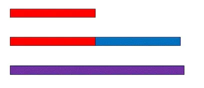
What happens if we break the time step of the discrete case in half, first increasing by 50%, and then taking the output of this process and increasing it an additional 50%? This still gives 100% growth, but broken up into pieces. After this process; we have a final amount of

$\left(1+\frac{1}{2}\right)\left(1+\frac{1}{2}\right)1=\frac{3^2}{2^2}=\frac{9}{4}$

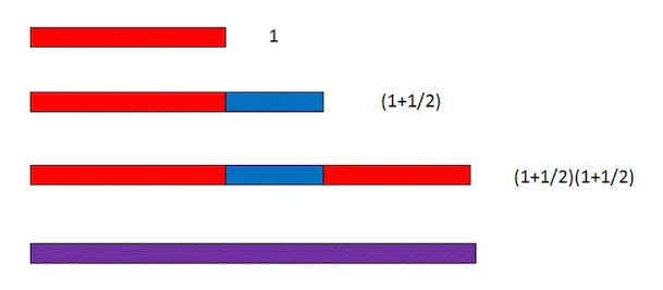
Which is greater than the unbroken doubling which results in 2. What about breaking the time step into three pieces, and growing at a rate of 1/3 over each period? The result of this process is below:

$\left(1+\frac{1}{3}\right)\left(1+\frac{1}{3}\right)\left(1+\frac{1}{3}\right)1\approx 2.37$

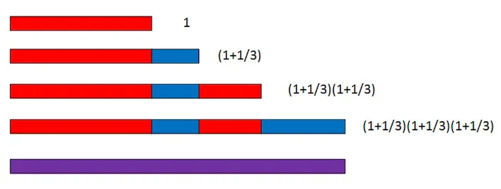
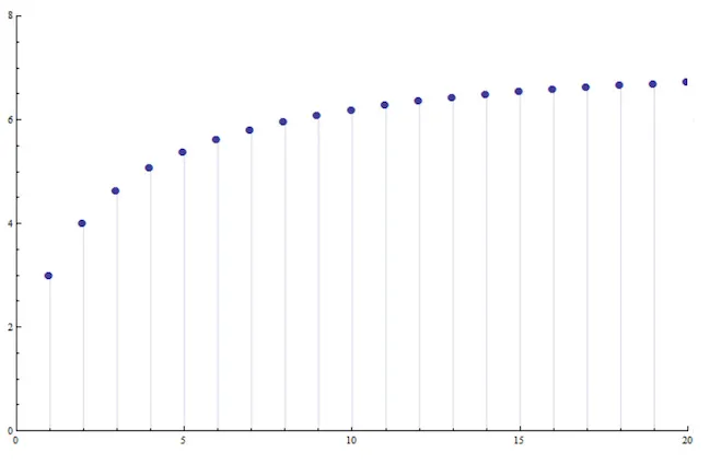
This is even larger than the previous division, which raises a question: does dividing 100% growth over the unit time interval diverge as the number of divisions tends towards infinity? If we divide the unit time interval into n pieces, and grow at a rate of 1/n during each step; we reach a final value of

$\left(1+\frac{1}{n}\right)\left(1+\frac{1}{n}\right)\left(1+\frac{1}{n}\right)\cdots \left(1+\frac{1}{n}\right)$

For n=100, here are the bars analogous to those above

As the bars get more numerous, exponential growth begins to appear. Changing the value of n does not add more terms to the end of this sequence, but rather refines the sequence, making each individual bar smaller. The limit of these bars to zero width is then the model of continuous 100% growth that we are seeking. Looking over a wide range of n values, it appears that the value after unit time is tending towards a fixed number. Assuming this indeed happens, then breaking 100% growth into pieces and distributing it over smaller and smaller intervals results in a value of

$\lim_{n\to\infty}\left(1+\frac{1}{n}\right)^n$

after one unit time step. But this is exactly the same limit we originally discovered with differentiation, just disguised! Recall there $e=\lim_{h\to 0}\left(1+h\right)^h$ Replacing $h$ with $1/n$ means as $h\to 0$ we must have $n\to\infty$, and this limit transforms into our newfound one. Thus, the constant of continuous growth is exactly the same found this way, as via calculus.

The Utility of $e$ as a base

We have come across a few different mathematical reasons that select e as a rather special base for the exponential function; but it’s most useful property is yet to come. If e represents the result of continuous 100% growth, what is the result of 50% continuous growth over an interval? Looking back at the above limit for e, we can see that breaking the original 100% up over n time steps resulted in the formula

$\left(1+\frac{1}{n}\right)^n$

Likewise, distributing 50% growth over n time steps would produce a final result of

$\left(1+\frac{0.5}{n}\right)^n$

Lets take a quick look at what this converges to as $n\to\infty$, this comes out to approximately 1.6482. Is it a coincidence that this is precisely the square root of e? Definitely not! Let’s see why: To get to the limiting value of this expression; we don’t need to consider all the terms; the limit just asks what happens “at infinity”, so as long as we consider at least some of the terms way out there; we can see what happens (this can be made more precise by noting that since the original sequence is convergent, so are its subsequences). Before jumping into the whole subsequence stuff, lets just look at a relatively “big” term, by setting $n=50$.

$\left(1+\frac{0.5}{50}\right)^{50}$

We can re-write this as follows:

$\left(1+\frac{0.5}{50}\right)^{50}=\left(1+\frac{1/2}{50}\right)^{50}=\left(1+\frac{1}{100}\right)^{50}=\left(1+\frac{1}{100}\right)^{100/2}$

The last term in this sequence looks a lot like one of the terms from our original sequence for e, except the exponent is divided by two. To make sure what we are witnessing here is something real and not just a coincidence; lets consider a much larger term: $n=5000$.

$\left(1+\frac{0.5}{5000}\right)^{5000}=\left(1+\frac{1/2}{5000}\right)^{5000}=\left(1+\frac{1}{10000}\right)^{5000}=\left(1+\frac{1}{10000}\right)^{10000/2}$

This time we end up with the 10,000th term in the sequence for $e$ (except we also have that factor of $1/2$ in the exponent). Using what we know about fractional exponents however, raising something to the half power is the same as taking the square root. So these are just the square root of two terms in the sequence for $e$. If this pattern continues; then we can show that the base for continuous 50% growth is really just the root of $e$, as was suggested numerically.

This is a remarkably useful fact: the base of the exponential which represents 50% continuous growth is simply $e^{0.5}$. More generally, continuous growth at a given rate has for an exponential base $e^{\mathrm{rate}}$. Using the above argument as a guide, we can show this rather simply. For a given $r$, which we will interpret as the growth rate, we will construct a sequence of terms limiting to continuous growth at rate $r$. Like before, we will go about this by dividing $r$ evenly over the unit interval and limiting to infinity, producing the sequence

$\lim_{n\to \infty}\left(1+\frac{r}{n}\right)^n$

Here’s a plot of the terms of this sequence for some example value of $r$:

Actually computing this limit by hand for arbitrary $r$ is challenging, so we perform a little trick. Since the natural numbers are just points along the number line, we can extend our limit from just being over $n$ to being over real numbers $x$ as $x\to\infty$:

$\lim_{x\to \infty}\left(1+\frac{r}{x}\right)^x$

Here’s a plot f the continuous extension:

Our original limit is a subsequence of the continuous limit, and so we can choose a different subsequence if we would like and be guaranteed that it will converge to the same limit (since the overall continuous limit exists here). To choose a different discrete subsequence, instead of counting upwards by integers, lets count upwards by multiples of $r$. The new variable in the limit will then be $rm$ for $m$ an integer.

$\lim_{m\to \infty}\left(1+\frac{r}{rm}\right)^{rm}$

Here’s a plot of the continuous curve resampled at these new points

Now, we just have to compute this limit in terms of things we already know, and our earlier example with $r=0.5$ provides a guide. Indeed cancelling the $r$s on the inside fraction,

$\lim_{m\to \infty}\left(1+\frac{r}{rm}\right)^{rm}=\lim_{m\to \infty}\left(1+\frac{1}{m}\right)^{rm}=\left[\lim_{m\to \infty}\left(1+\frac{1}{m}\right)^{m}\right]^r$

But we know the quantity in the brackets is $e$! So, this limit is precisely $e^r$. Although it was a lot of work to reach this step; it was well worth it. This provides possibly the single most compelling reason that $e$ shows up everywhere: it is not only the base representing 100% continuous growth, but continuous growth at any rate can be represented simply in terms of it, by simply raising $e$ to the power of that rate! Out of all possible exponential bases, $e$ is the only one with this property. It definitely makes sense to call $e$ the “natural” base.

Differentiation of Exponentials

It is again due to the properties of e that we have such simple formulas for the derivatives and integrals of an exponential function. The simplest case of course, is just that of $e^x$, where we have the nice formula $\frac{d}{dx}e^x=e^x$ Because all exponentials can be written simply as stretched copies of this curve, we need not even consider how to differentiate them individually. Instead, we can just focus on the derivative of $ae^{bx}$, knowing that we can determining the appropriate values of the constants using some of our previous arguments. This is of course nothing more than a simple exercise of the chain rule; but we will try and go about it somewhat differently to develop some intuition.

The derivative of a function measures it’s rate of change in the vertical with respect to the horizontal (thus the notation $dy/dx$), so the effect of a vertical stretch is simple to understand. If we multiply a function by a constant $a$, then we have replaced the y coordinate of each point on the graph with a point $a$ times farther from the x-axis, but we have left the x coordinate unchanged.

If we view the derivative as the change in y relative to the change in x, we note that y changes a times as fast as before, whereas x changes at the same rate. Thus we would expect the change of our new function to be $a$ times greater than before. In symbols; this is one of the properties that makes the derivative a linear operator: $\frac{d}{dx}\left(af(x)\right)=a\frac{d}{dx}f(x)$ In the case of our exponentials, a vertical stretch equates to starting with a different initial amount. The above property can then be interpreted as saying that starting with an amount a causes the rate of change of your function to be a times greater than before. This makes perfect sense in our scheme due to the already-noted fact that exponential growth is characterized by the growth being proportional to the amount available. Since there is a times as much stuff, then it grows a times as quickly.

Now what about a horizontal stretch? Going back to thinking of the derivative as a limit of the ratio “y-change to x-change”, we can see that a horizontal stretch leaves the y-coordinate unchanged, but stretches the x-coordinate. If we compress the x-coordinate by a factor of 2, then all of the y-coordinates will be brought twice as close together: that is our x-interval will be half the size that it was before the compression.

Because we are looking at the ratio y-change to x-change, if we fix our y-change to be the same, then our x-change is half of what it was, and the ratio is doubled (there was a 1/2 in the denominator). In general, if we stretch our x axis by a factor of $b$, then for the same y-change, we have an x-interval which is $1/b$ as large; making our new ratio $b$ times the old. In symbols; this is the chain rule for constant coefficients: $\frac{d}{dx}f(bx)=bf'(bx)$ Let’s apply this reasoning to exponentials: a horizontal stretch of magnitude $b$ is equivalent to a change of base in general. However, if we choose the base $e$ to begin with, then a horizontal stretch of $b$ can be re-interpreted as the rate of continuous growth. Applying the above rule for the natural exponential $\frac{d}{dx}e^{bx}=be^{bx}$ This simply says that if something is continuously growing at rate $b$, then its growth at time $t$ is equal to that rate times the amount currently available.

From this we can construct a formulation for the derivative of a general exponential : a simple horizontal stretch will allow us to write this exponential with base e. As was discussed before, the inverse function of $e^x$ will provide us with the correct stretch. $a^x=e^{\log_e(a)x}$ Where, to stick with the standard notation in calculus we will write $\log_e$ as $\ln$. This provides us with useful information even beyond just the ability to take the derivative, saying that something grows at rate is the same as saying it grows with rate $\ln(a)$. This interpretation of all different exponential bases simply being horizontal stretches of the natural base also gives us the following form of their derivative $\frac{d}{dx}a^x=\frac{d}{dx}e^{\ln(a)x}=\ln(a)e^{\ln(a)x}=\ln(a)a^x$ which just says the rate of change is the growth rate times the current amount.

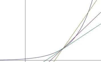
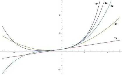
Computationally, one of the main advantages of $e^x$ lies in the fact that it is its own derivative. From this its easy to see that the second derivative of $e^x$ is also itself, as is the 3rd or any higher derivative. Most notably, every derivative takes the value 1 at x=0. To see why this is useful, consider the Taylor series of a general function $f(x)$. If $f$ is analytic, we can express it in the form $f(x)=\sum_{n=0}^\infty \frac{f^{(n)}(0)}{n!}x^n$ Using the fact that $f^{(n)}(0)=1$ for all $n$ when $f(x)=e^x$, we see that $e^x$ is the function with the simplest Taylor series: $e^x=\sum_{n=0}^\infty \frac{1}{n!}x^n=1+x+\frac{x^2}{2}+\frac{x^3}{6}+\cdots$ The plot below shows the convergence of the first 4 terms in this series towards the exponential:

This provides us with yet another means of calculating the value of e; one that turns out to be quite efficient: setting x to 1 in the above formula yields $e=\sum_{n=0}^\infty \frac{1}{n!}=1+\frac{1}{2}+\frac{1}{6}+\frac{1}{24}+\frac{1}{120}+\cdots$ which is much simpler to compute than the previous limiting definitions.

Although more difficult to think about intuitively, this Taylor Series may be taken as the definition of $e^x$ if you like. In fact, it is one of the most useful definitions to keep around, because it is easy to extend the meaning of the exponential to other domains, (e.g. what does e to the power of a matrix mean? e to a differential operator? e to the imaginary unit?) but we wont deal with it much here, extending the domain of the exponential via the approach “plug it into the taylor series and see what comes out” doesn’t really provide much intuition behind why the extension behaves the way it does.

Summary

We’ve covered a ton of information here, so it’s probably a good idea to highlight the important bits (plus, this will show you how far we’ve come!)

• The “laws of exponents” themselves are just a consequence of our notational choice; namely “exponentiation is just a shorthand for repeated multiplication”.
• Negative exponents are a shorthand for repeated division
• Reciprocal exponents (of the form 1/q) are another notation for the qth root.
• Shifting an exponential horizontally is equivalent to vertically stretching it
• Changing the base of an exponential is equivalent to horizontally stretching it
• The unit base for discrete growth is 2.
• The unit base for continuous growth is e
• Starting with amount A and growing continuously at rate r is modeled by
• The exponential with base e is equal to its own derivative precisely because the proportionality constant between current amount and growth rate is 1.