The Fourier Transform

Decomposing functions the same way you decompose vectors — just in infinite dimensions.

Fourier series and the Fourier transform both give us ways of expressing different functions in a radically different way - instead of looking at a function for how it depends on the input $x$ - we look to see how it decomposes into basic oscillations at different frequencies.

My goal here is not to be rigorous, but to give some explanation and intuition for why the formulas defining the Fourier series coefficients and the Fourier transform have the form they do - as this was somewhat mysterious to me during my first pass at Fourier analysis.

The Goal

Fourier analysis began with Joseph Fourier’s realization that $2\pi$ periodic functions could be written as an infinite sum of sines and cosines: $f(x)=\frac{a_0}{2}+\sum_{n=1}^\infty a_n \cos (n x)+\sum_{n=1}^\infty b_n\sin(nx)$ With the coefficients given by the following formulas:

$a_0=\frac{1}{\pi}\int_{-\pi}^\pi f(x)dx$
$a_k=\frac{1}{\pi}\int_{-\pi}^\pi f(x)\cos(xk)dx$
$b_k=\frac{1}{\pi}\int_{-\pi}^\pi f(x)\sin(kx)dx$

To make the similarity clearer with the Fourier transform however, we will take a more modern viewpoint and use the identity $e^{ix}=\cos(x)+i\sin(x)$ to write things a bit more succinctly:

$$f(x)=\sum_{k=-\infty}^\infty c_k e^{ikx} \hspace{2cm} c_k=\frac{1}{\pi} \int_{-\pi}^\pi f(x)e^{-ikx}dx$$

The Fourier transform gives a pairing between certain non-periodic functions on the real line: any function $f(x)$ whose square is integrable has a fourier transform, denoted $\mathcal{F}(f)=\hat{f}(k)$ defined by

$$\mathcal{F}(f)=\hat{f}(k)=\frac{1}{2\pi}\int_{\mathbb{R}}f(x)e^{-ikx}dx \hspace{2cm} \mathcal{F}^{-1}(\hat{f})=f(x)=\int_{\mathbb{R}}\hat{f}(k)e^{ikx}dk$$

Our goal, is to figure out what these formulas mean, and where they came from.

In Words

Let’s begin by trying to read these formulas in words. One formula from each pair isn’t that bad: looking at Fourier series first, $f(x)=\sum_{n=-\infty}^\infty c_n e^{inx}$ says that any periodic function $f(x)$ can be written as an infinite sum of complex exponentials (sines and cosines) with different coefficients (think of these as “weights”) on each. While perhaps unbelieveable (what?! you can write every periodic function as a sum of nice smooth oscillations?!) its at least an understandable claim.

The same holds for one of the formulas from the Fourier transform pair: $f(x)=\frac{1}{\sqrt{2\pi}}\int_{\mathbb{R}}\hat{f}(k)e^{ikx}dk$

This says that every square integrable function on $\mathbb{R}$ is actually the integral of some other function against a complex exponential. But interpreting the integral as a continuous sum, this has the same content as the formula above: it says every function may be written as a sum of weighted complex exponentials.

Ok, so what about the weights? According to our interpretation above, the numbers $c_k$ and $\hat{f}(k)$ are supposed to tell us what weight we should assign $e^{ikx}$ as a component of $f(x)$:

$c_k=\frac{1}{\pi}\int_{-\pi}^\pi f(x)e^{ikx}dx$ $\hat{f}(k)=\frac{1}{\sqrt{2\pi}}\int_{\mathbb{R}}f(x)e^{-ikx}dx$

These also appear to say the same thing in spirit: the amount of the $k^{th}$ frequency ($e^{ikx})$ in the function $f(x)$ is given by some multiple of an integral of $f$ against $e^{-ikx}$. But why should this measure the amount? It turns out there’s a good reason, and to see it - let’s take a detour into linear algebra!

Vectors and Bases

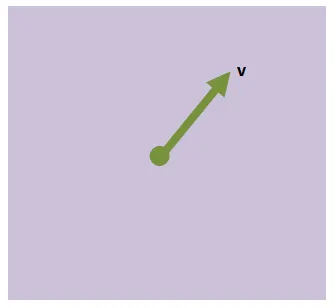
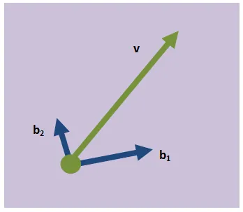
To keep things simple, lets start out with a vector in . Call this guy $v$. Without choosing a basis, we don’t have any convienent way to express $v$ other than by its name.

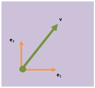
To help us easier express $v$ and other vectors we might care about, let’s bring a set of basis vectors into our picture. For now, let’s stick to the standard basis $e_1=(1,0)$ and $e_2=(0,1)$.

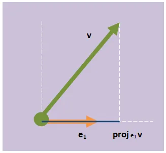
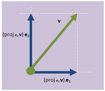
To write v in terms of them, we need a way to somehow say “how much” of $v$ is in the direction of each. Let’s look at how to do this for $e_1$. Let’s say for a second we have a “projection” operation, which takes v and “squishes it down onto $e_1$. We will call this $\textrm{proj}_{e_1}(v)$. Now lets do the same for $e_2$. We now have the “amount” of $v$ in the direction of each of our basis vectors, so how do we go about using this information to describe the vector? Well, we used the projection operation and the basis to “take our vector apart”, so let’s put it back together! Multiplying each basis vector by the projection amount gives us two vectors, and adding these guys together gives us $v$ back.

In symbols, $v=\textrm{proj}_{e_1}(v)e_1+\textrm{proj}_{e_2}(v)e_2$. For now, we will do away with the projection notation, and simply refer to the components as the first and second components of $v$. That is, we will say that $v=v_1e_1+v_2e_2$, which is often abreviated $v=(v_1,v_2)$.

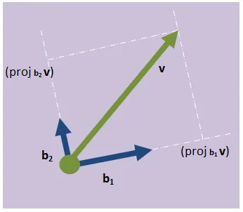
So, we have a nice coordinate representation of our vector, which we were able to construct by projecting our vector onto each basis vector individually. Now, what happens if we don’t find the “standard” basis particularly convenient for our problem; and we would like to look at $v$ from a different perspective? Well, we can always just choose a new one, say this basis:

(throughout this, we are only going to consider orthogonal bases, because that is all we will need to make the analogy with the Fourier Transform). We want a representation of our vector in terms of this basis? No problem; we can just project $v$ onto each one like before.

This lets us express $v$ in a new way: $v=\textrm{proj}_{b_1}b1+\textrm{proj}_{b_2}b_2$, which we could write as $v=\tilde{v}_1b_1+\tilde{v}_2b_2$ or $v=(\tilde{v}+1,\tilde{v}_2)$ if the basis was understood.

These two descriptions of our vector have different numerical values (as they should since each describes the vector in terms of the “amount” of it in a different direction), but there is no question they represent the same vector. From both representations it is simple to recover $v$, and in fact you can convert between the two representations with ease (think change of basis matrix).

Projections

Let’s take another quick detour and look at how to define the projection operator. We’ll look at two vectors, $u,v$ in $\mathbb{R}^2$ and determine how to project $v$ onto $u$.

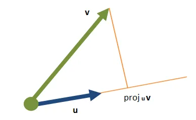
If we look at this as a triangle, we know the length of the hypotenuse (its just $|v|$), and the projection we want is the length of the bottom side. If we know the angle $\theta$ between $u$ and $v$; we can express this length as $\textrm{proj}_{u}v=|v|\cos\theta$ Convienently, this actually looks quite a bit like the geometric formulation of the dot product between two vectors. Recall that the dot product of two vectors satisfies the relationship $u\cdot v=|u||v|\cos\theta$ for $\theta$ the angle between them. Thus, our sought-after projection operator is none other than a rescaling of the dot product! $\textrm{proj}_u(v)=\frac{u\cdot v}{|u|}$ And so we’ve managed to kick the can down the road a little farther: we wanted to understand vectors so we wrote them as projections onto an orthogonal basis, then we wanted to understand projections so we wrote them in terms of the dot product. I bet you can guess what we have to take a look at now…

The Dot Product

As our goal is eventually to understand the formulas of Fourier, it will be helpful here if we don’t continue to restrict ourselves to $\mathbb{R}^2$. Lets say we have two vectors, $u,v$ in $\mathbb{R}^n$ which we can express in the standard basis as $u=(u_1,u_2,\ldots,u_n)\hspace{2cm}v=(v_1,v_2,\ldots,v_n)$ Their dot product is then given by the formula $u\cdot v=u_1v_1+u_2v_2+\cdots u_nv_n=\sum_{i=1}^n u_iv_i$ So, in a coordinate representation, we can say that the dot product is the sum of the products of each coordinate. There is one more important point here: we obviously want this new definition of the dot product to agree with the geometric one; and if we allow our vectors to be complex numbers, to accomplish this we need to take the complex conjugate of one of our vectors, replacing the above with this new definition: $u\cdot v=\sum_i u_i\bar{v_i}$ Where the overbar represents the complex conjugate. Obviously this definition reduces to the above if $v$ has all real components, but the only important part is that this is the “good” definition, in that it agrees with our geometric definition, and allows us to use the dot product to express projections. Now that we have a formula for the projection, let’s write out in full detail our decomposition of a vector into a sum of weighted basis vectors:

Just for the sake of being able to write things out explicitly, lets say that we know how to write $v$ in the basis $\{e_i\}$, $v=(v_1,\ldots, v_n)$ but we would like to be able to express it in another orthogonal basis $\{b_k\}$. Then

$v=\sum_k \tilde{v}_k b_k=\sum_k \textrm{proj}_{b_k}(v) b_k=\sum_k \left(\frac{v\cdot b_k}{|b_k|}\right)b_k$ where computing $v\cdot b_k$ according to the components in the basis $\{e_i\}$ we have $v\cdot b_k=\sum_i v_ic_i$ for $c_i$ the amount of $e_i$ in $b_k$.

The Vector Space of Functions

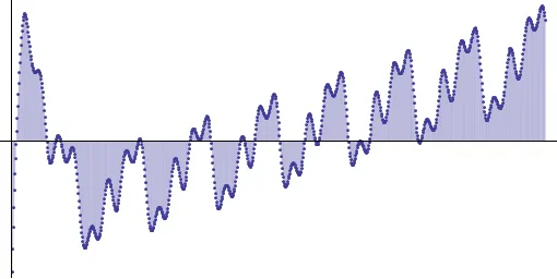
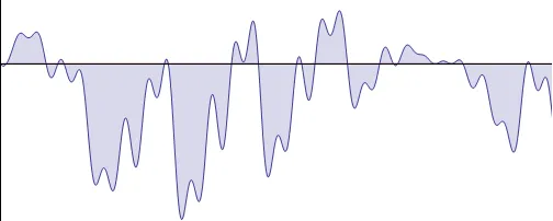
This detour into linear algebra is more applicable than it may have seemed at first - for our actual problem is taking place in a vector space! The space of functions from $\mathbb{R}\to\mathbb{R}$ is a vector space as we can add functions and multiply them by scalars - the only thing that differs from our usual experience is that its infinite dimensional! Here’s a vector in that space.

You can think of this graph as a “coordinate representation” of our function f. To each distance from the origin x, we can say the xth coordinate of f is f(x). It’s going to turn out that to make sense of fourier analysis we are going to need to project a function like this onto a basis of sinusoids, so we should first talk about the dot product for functions. To figure out the right generalization let’s return to familiar linear algebra in finite dimenisons. We defined the dot product of two vectors $u,v$ in $\mathbb{R}^3$ to be

$u\cdot v = u_1v_1+u_2v_2+u_3v_3$

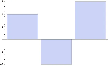
Take for example the vectors $u=(1,2,3)$ and $v=(2,-1,1)$. We can visualize this sum geometrically as an area: we make a bar-graph with three entires, one bar for each component, and the height of the $i^{th}$ bar is $u_iv_i$.

$u\cdot v = \sum_{i=1}^3 u_iv_i=(1)(2)+(2)(-1)+3(1)=3$

If we now go from 3D vectors to vectors of arbitrary length; the sum representing the dot product is made of more and more rectangles. Below we show three cases, 18 dimensional vectors 100 dimensional vectors, and 1,000 dimensional vectors.

$u\cdot v = u_1v_1+u_2v_2+\ldots +u_nv_n=\sum_{i=1}^n u_i v_i$

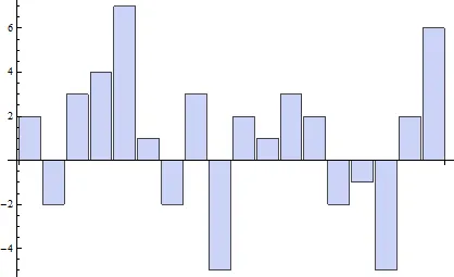
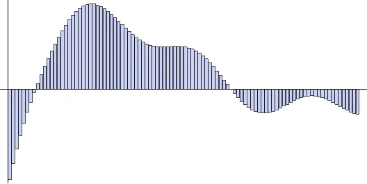
In each case the dot products value is the net area under this bargraph. So, what happens in infinite dimensions? Here, every single point on the horizontal axis represents a coordinate (the “xth coordinate of f”), and so we must sum over every coordinate — over a continuum. Just like before, this continuous sum becomes an integral. Thus, like the dot product of vectors is the sum of the products of the coordinates; the dot product of functions (usually called the L2 inner product) is the integral of the products of the values:

$f(x)\cdot g(x)=\int_{\mathbb{R}}f(x)g(x)dx$

However, we do have one more thing to clean up. This definition works fine in the real case, but for complex functions we need to make sure to take the complex conjugate (again, this is to make sure that the dot product still works how we want it to; that it lets us define a projection operator).

$f(x)\cdot g(x)=\int_{\mathbb{R}}f(x)\overline{g(x)}dx$

And finally, if we are working with functions on a bounded domain like $[a,b]$ instead of the real line, the integral only goes over these bounds (as this is the only spot where our functions “coordinates” $f(x)$ are defined). For us, the important case is periodic functions on $[-\pi,\pi]$, which has the dot product

$f(x)\cdot g(x) = \int_{-\pi }^\pi f(x)\overline{g(x)}dx$

Projecting a Function onto a Basis

Now we are ready to really build the idea of fourier analysis. Starting with a function $f(x)$ thought of as an infinite dimensional vector

We want to write it in a basis - as a nice weighted sum of simple functions. And here, the simple functions are going to be oscillations. One could choose to use a basis of sines and cosines for the oscillations,

But we know the complex exponential is a better choice: it combines both into one, making our formulas shorter:

$e^{ix}=\cos(x)+i\sin(x)$

Different frequencies of oscillation are modeled by changing the angular frequency of the sinusoids, so $e^{ikx}$ for various values of $k$. Following what we did above then, if we were to try break a function up into its component frequencies (modeled by the functions $e^{ikx}$) we would write something like this:

$f(x)=\sum_k f_k e^{ikx}=\sum \textrm{proj}_{e^{ikx}}(f)=\sum_k\left(\frac{f(x)\cdot e^{ikx}}{|e^{ikx}|}\right)e^{ikx}$

Of course, there are many things we need to make sense of in this formula still, but bear with me. First off, this sum is infinite as we had said above, but is it discrete or continuous (is it an honest sum, or an integral)? Well, that all depends on how many different frequencies we need to describe our function. If we are talking about a periodic function, much like a guitar string can only play discretely many sounds (it can either vibrate with zero, one, two, … nodes), there are only discretly many oscillations with that given period

Thus, in that case our sum will just be over the integers (representing how many times the function vibrates within the interval) and we have this to make sense of. $f(x)=\sum_{k=-\infty}^\infty \left(\frac{1}{|e^{ikx}|}(f(x)\cdot e^{ikx})\right)e^{ikx}$ However, if we are not looking at periodic functions but instead at all functions on the real line, there is no restriction on the period! All functions of the form $e^{ikx}$ could contribute, and so we expect to have to sum up over a continuum of contributions, making it into an integral: $f(x)=\int_{\mathbb{R}} \left(\frac{f(x)\cdot e^{ikx}}{|e^{ikx}|}\right)e^{ikx} dk$ is what we should try and interpret.

In each case, this leaves us with two things to fill in: a value for $|e^{ikx}|$ and an expression for $f(x)\cdot e^{ikx}$. Luckily we already figured out how dot products work in infinite dimensions, they involve integration and complex conjugation. And as the complex conjugate of $e^{ix}$ is none other than $e^{-ix}$ we can see that depending on which case we are considering, the dot product $f(x)\cdot e^{ikx}$ is one of the below:

$\int_{-\pi}^\pi f(x)e^{-ikx}dx\hspace{2cm}\int_{\mathbb{R}}f(x)e^{-ikx}dx$

Which are almost identical to the formula for the Fourier transform and the coefficients of the fourier series! All we are missing is a normalization constant - which reminds us, we have forgotten still one part of the definition of the projection: $|u|$- the size of the vector you are projecting onto. It turns out that in the periodic case it works out best to think of the “size” of $e^{ikx}$ to be $\pi$, and in the non-periodic case, where its domain is all of $\mathbb{R}$, to be twice that. (There are better explanations for why these values are what they are, but I’m just trying to tell a memorable story here).

Thus, we have completely recovered the formulas for the Fourier coefficients - they are just the projections of our functions onto functions of the form $e^{ikx}$ - it really is just linear algebra (albeit of the infinite-dimensional variety).

Visualizing the Projection

It turns out that the integral defining the projection here has a rather pretty interpretation I’d like to share quick before ending - remember that we can think of $e^{ikx}$ as a point spinning around counterclockwise on the unit circle, at constant speed k:

The complex conjugate, $e^{-ikx}$ is just the clockwise version of this.

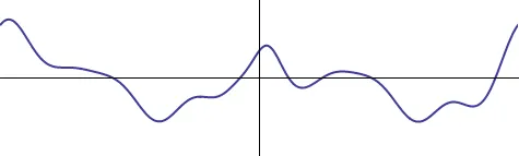
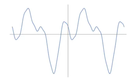
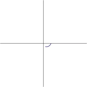
Remember that our projection integral is of the form $\int f(x)e^{-ikx}dx$, where $f(x)$ is a real valued function - so the integral is just the polar form of a complex number: the distance from the origin is $f(x)$ and the angle with the real line is $kx$! It’ll be easiest if we do an example. Consider the $2\pi$ periodic function $f(x)=3\sin(x)+2\cos(2x)-2\sin(3x)+\frac{1}{5}\cos(10x)-sin(2x)$

Multiplying this by $e^{-ix}$ corresponds to spinning it about the origin in $\mathbb{C}$ at unit speed:

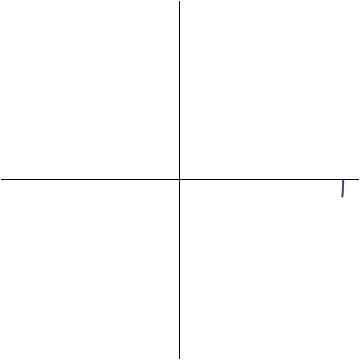
Integrating this over one period adds up all of the directions, weighted by the magnitude in that direction: the final answer is a vector in the plane (a complex number) representing the average direction that the spun-out curve points in $c_1=\frac{1}{\pi}\int_{-\pi}^\pi (3\sin(x)+2\cos(2x)-2\sin(3x)+\frac{1}{5}\cos(10x)-sin(2x))e^{-ix}dx$

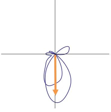
The net contribution of angular frequency 1 can then be seen to be represented by an arrow along the negative imaginary axis. The magnitude of this arrow tells us the amplitude of the contribution, and its phase (90 degrees from the real axis) tells us that the contribution is sinusoidal.

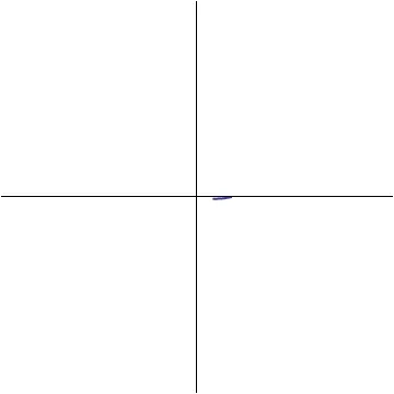
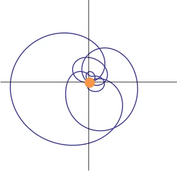
If sinusoidal contributions are represented by vectors along the imaginary axes, lets look at a cosinusoidal contribution: we will spin the function at an angular speed of 10 to single out the cosine at that frequency:

Adding up all the vectors along this spinning process yeilds the average, which is the projection $c_{10}=\frac{1}{\pi}\int_{-\pi}^\pi (3\sin(x)+2\cos(2x)-2\sin(3x)+\frac{1}{5}\cos(10x)-sin(2x))e^{-10ix}dx$

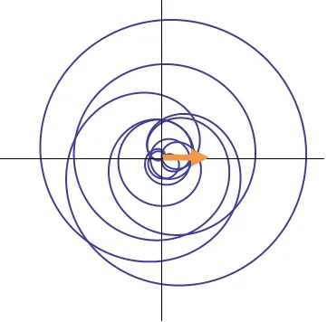
Thus, as we should have expected, the net effect is a smaller arrow along the real axis, representing zero initial phase.

Yet another case we can investigate is that of angular speed 2. In our formula, we have both sinusoidal and cosinusoidal oscillations at that frequency. From elementary trigonometry we know that the sum of these two is a single oscillation with an initial phase shift. For illustrative purposes, let’s perform our projection onto this frequency and see.

$c_2=\textrm{proj}_{e^{2ix}}(f(x))=\frac{1}{\pi}\int_{-\pi}^\pi (3\sin(x)+2\cos(2x)-2\sin(3x)+\frac{1}{5}\cos(10x)-sin(2x))e^{-2ix}dx$

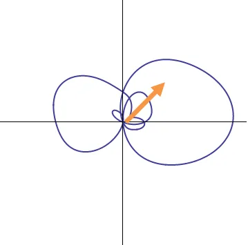
The net contribution is found to be phase shifted at 45o, representing a combination of both real (cosine) and imaginary (sine) components.

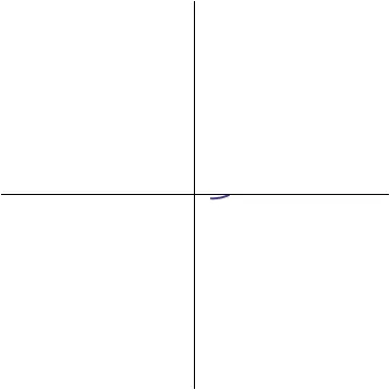
There’s still one more thing we can check out with this example: what if we spin our function at angular frequency 4? Looking back at the original function, there is no oscillations at that frequency present; so we expect the Fourier component at that frequency to be 0.

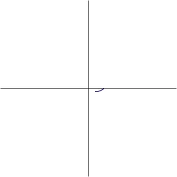
While the graph certainly moves farther out to the left, it spends more time on the right. And when we carefully add it all up to get the projection, we find precisely zero:

Summary

Here’s what I hope you take away from this article:

• Functions can be decomposed into frequencies, much like vectors can along bases
• The contribution of each frequency to a function is the projection of that function on the frequency
• Projecting on a frequency is accomplished by spinning the function at that frequency, and looking at the net effect
• The set of contribution amounts for each frequency in a function is called its Fourier Transform
• Re-constituting a function from its frequency components is called the Inverse Fourier Transform
• We can look at the coordinate representation and the frequency representation as two ways to get information about the same function; and we can look at their values as being the components in two different “bases”