The Gradient

Developing the gradient from directional derivatives and contour maps.

The gradient is a kind of higher-dimensional version of the derivative we are used to from one dimensional calculus. Before getting started, let’s take a minute to review the “normal” derivative of 1-d functions to give us an analogy to work with. When we talk about derivatives, we are talking about the rate of change, or the slope of the tangent line to our function. Given a point x, the derivative of our function at that point tells us how quickly it is increasing or decreasing there.

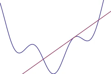
We usually picture this rate of change as the slope of the tangent line to the graph at that point, and so we can think of the derivative as a function that takes in points and spits out slopes

$\frac{d}{dx}\colon(\mathrm{point})\mapsto (\mathrm{slope})$

A useful way to think of the derivative is like a level. When you set a level on a bookshelf before securing it to the wall, you are measuring how far the bookshelf deviates from horizontal, that is, its rate of change in the vertical direction. Now picture putting a level on the above graph at the point we have the tangent line drawn. The little bubble inside would rise to the right, indicating a positive slope, or a positive derivative.
Now derivatives are such a nice thing to have lying around for one-variable functions, so it would be pretty sweet if there was a nice way to generalize them to real functions of two or more variables. To keep all the visualizations simple, we will only talk about real functions of two variables here, which can be pictured as surfaces above a plane (much like the graphs of 1-d calculus can be visualized as curves above a line).

Of course, all of the things we will say about two variable functions extend to the higher dimensions, so we aren’t losing anything by sticking to the case that’s easy to visualize. The reason for this is that the single variate functions are quite different from all their higher-dimensional cousins in that there is only one “direction to change in” at any given point. Seeing this difference is easy if we go back to the level analogy. Picture the graph of a single variable function as being the very top ridge of a mountain, and say you are hiking along the ridge with a level in hand.

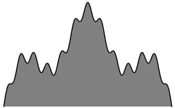
When you reach a certain point on the horizontal axis, say I yell up to you “Hey! What is the slope of the mountain ridge where you are?” And, without any further information from me, you could lay the level down tangent to the ridge, and look at where the bubble goes. “Looks like a slope of 10 deg upwards!” you might yell back after reading your level, and I would be able to interpret this easily, as I can see where you are and there is only one direction to walk along the ridge. Contrast this with the two dimensional case, where now instead of walking along a ridge, you are walking through a hilly mountain valley.

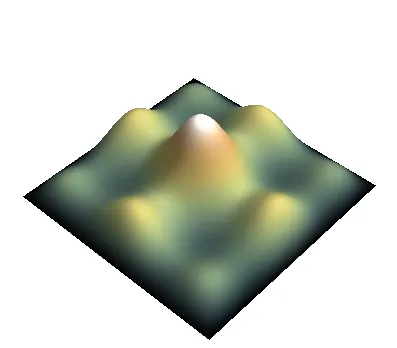
If you were standing at a particular point and I ask you what the slope is, you might very well lay down your level (maybe in the direction you were walking) and shout it’s reading back to me. This seems all good, just like in the 1-d case, we can use the level to convert points to slopes. However, there is not a single direction in which to measure slope here on the surface, but instead there’s infinitely many! No matter which way you turn while standing at that point, you could lay your level down and take a reading, thus giving a value for slope at that point. To see that these slopes definitely don’t need to be the same, let’s say there is a network of hiking paths on the mountain, which criss-cross at certain points.

$(\mathrm{Point},\mathrm{Direction})\mapsto \mathrm{Slope}$

Since there are many directions you could move starting at a single point, we’d like to collect all of these slopes (in math-speak, directional derivatives) together, and have a mathematical object attached to each point which stores the slope in every direction. This seems to be a good generalization of the single variate derivative to higher dimensional functions, because the 1-d version also stores the slope in all directions: it just so happens that there is only 1 direction to start with! Given a 2-dimensional function f, we will refer to it’s derivative (or collection of all it’s directional derivatives) as the gradient of f, written $\nabla f$.

To say that this derivative “stores” all the directional derivatives, what we mean is that given the gradient and a direction, we can immediately recover the slope of our function in that direction. In slightly more mathy terminology;

$\left\{\nabla f, v\right\}\mapsto D_v f$

This gives us a little insight into what kind of an object the gradient itself might be (notice, until now we really don’t know; from the definition we gave it might very well be a gigantic list of every possible directional derivative!). Since given a vector and the gradient, we want to get back the slope (a scalar), the gradient must be some object that when combined with a vector can give a scalar. If the gradient were also a vector, we’d have exactly what we need, as the dot product of two vectors is a scalar! This gives us a new, more precise definition of the gradient. The gradient is the unique vector field such that its projection along any direction is precisely the directional derivative in that direction. The equation specifying this vector field implicitly is

$\nabla{f}\cdot v = D_vf$

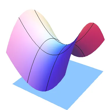
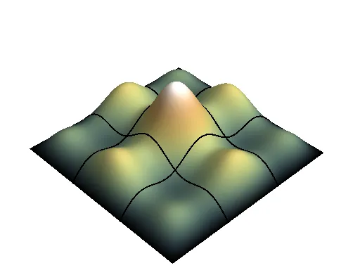
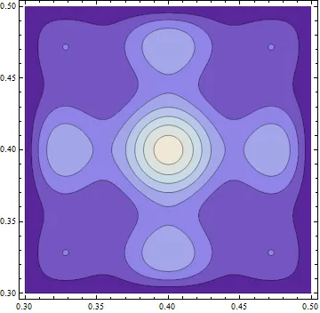
So, at least we know how to picture the gradient; for a 2 dimensional function it will appear as a bunch of arrows in the plane. In fact, we can do much better than that, because the gradient must encode all of the partial derivatives by design, its vector field has a very particular and easy-to-interpret shape: the gradient field always points uphill. Below is a picture of a function and its gradient to illustrate this, and we will make the claim more precise in a bit.

To see why this is how the gradient behaves, its useful to think about contour maps. When going hiking, it’s often useful to consult a contour map to give you an idea of the level of the land. These maps display lines of constant elevation; and the spacing between the lines gives you an idea of how steep the landscape is.

Wherever you’re standing on this landscape, there is a “contour line” which is the line of constant elevation (picturing yourself on a mountainside facing the peak, to your left and right will be the directions of constant elevation, and walking along this contour would not get you farther up nor farther down the mountain). Since along contour lines the change in height is zero, this means the directional derivative along the contour is zero. Mathematically, if v is in the direction of a contour line, $D_v(f)=0$. . But, we know that the dot product of the gradient and the direction is by definition the directional derivative, so we have $\nabla f \cdot v = 0$. Whenever a dot product of two vectors is zero, we know the two vectors are perpendicular. This tells us another very useful property of the gradient:

The gradient is everywhere perpendicular to the contour lines of a function

Thinking of yourself as on a mountain again, its easy to see that the direction of no incline is perpendicular to the direction which leads directly up/downhill. So, this tells us that the gradient vector must point either in the direction of greatest increase of the function, or in the direction of greatest decrease. To see that it in fact points in the direction of greatest increase, picture yourself on the mountainside facing directly towards the peak. The slope in the direction your facing is obviously positive, as its towards the top of the mountain. Let’s say that this direction is given by the vector u. Then the directional derivative in u’s direction should be positive, and in fact should be the maximum value of any directional derivative (if you turned yourself at any other angle than directly uphill, the slope upwards would be less). This tells us that $\nabla f \cdot u = \mathrm{max}$ which we know from the properties of the dot product in linear algebra, means that the gradient vector and u are parallel. Since we chose u to be the vector pointing in the direction of greatest increase, this gives us another useful property of the gradient:

The gradient points in the direction of greatest increase of the function at each point

Further, as we know that , and as u is parallel to the gradient, the magnitude of the gradient is just the value of this directional derivative (the maximum directional derivative at that point). This gives the last property we need to characterize the gradient geometrically.

The magnitude of the gradient is the value of the maximum directional derivative at the point

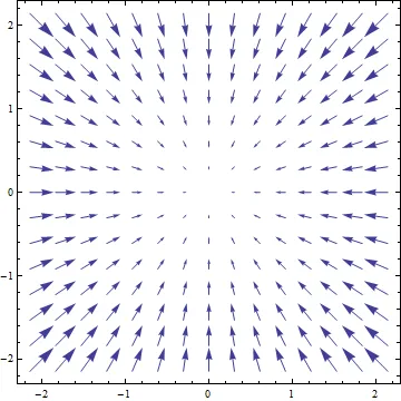
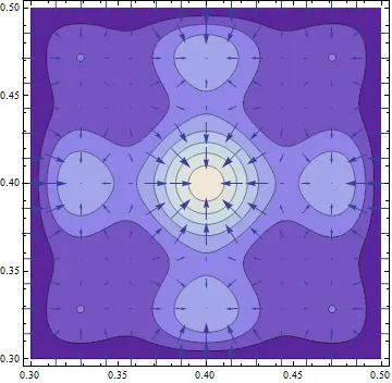
The graphic below shows the contour plot from the above function superposed with the gradient vector field. You can see the gradient is always perpendicular to the contours, pointing uphill, and the vectors scale in size with the steepness of the landscape, just as we had argued.

Calculating the Gradient

At this point, we have two useful characterizations of the gradient, which are good to keep in mind, but don’t help us much in way of computing the gradient of a function explicitly:

• The gradient is the unique vector field whose projection onto any direction gives the directional derivative
• The gradient is the vector field which points in the direction of the fastest increase of the function, whose length is the rate of increase in that direction

However, it would be nice computationally to have a formula for the gradient, which would allow us to compute it easily. Luckily, such a formula can be derived quite easily from our first characterization. In order to have a nice description of the gradient field, we need to choose a coordinate system to work in, and to keep things simple we will stick with Cartesian coordinates. Here, we have two basis vectors; one parallel to the x-axis and one to the y-axis, each of unit length. We want to express the gradient in this basis, meaning we want to write something like

$\nabla f = a e_1 + b e_2$

Because $e_1=(1,0)$ and $e_2=(0,1)$ are an orthonomral basis, it is easy to calculate the components $a,b$. The x-component of the gradient is simply it’s projection on to the vector e1, and the y-component is it’s projection onto e2, or more mathematically, $a=\nabla f\cdot e_1$ and $b=\nabla f \cdot e_2$. But, from the very definition of the gradient, we know that the projection onto the x-axis direction vector is the directional derivative along x, and the projection onto the y-axis is the directional derivative along y. In cartesian coordinates, these two directional derivatives have special names; they are the partial derivatives of f with respect to x and y. That is,

$a = \nabla f \cdot e_1 = D_{e_1}f=\frac{\partial f}{\partial x}$ $b = \nabla f \cdot e_2 = D_{e_2}f=\frac{\partial f}{\partial y}$

Which gives us our coordinate representation: it turns out the gradient is simply the vector consisting of the partial derivatives along each coordinate axis!

$\nabla f = \left(\frac{\partial f}{\partial x},\frac{\partial f}{\partial y}\right)$