Realizing Right-Angled Hyperbolic Hexagons in the Upper Half Plane

Turning abstract moduli data into concrete coordinates for rendering.

Here’s a link to the original computation

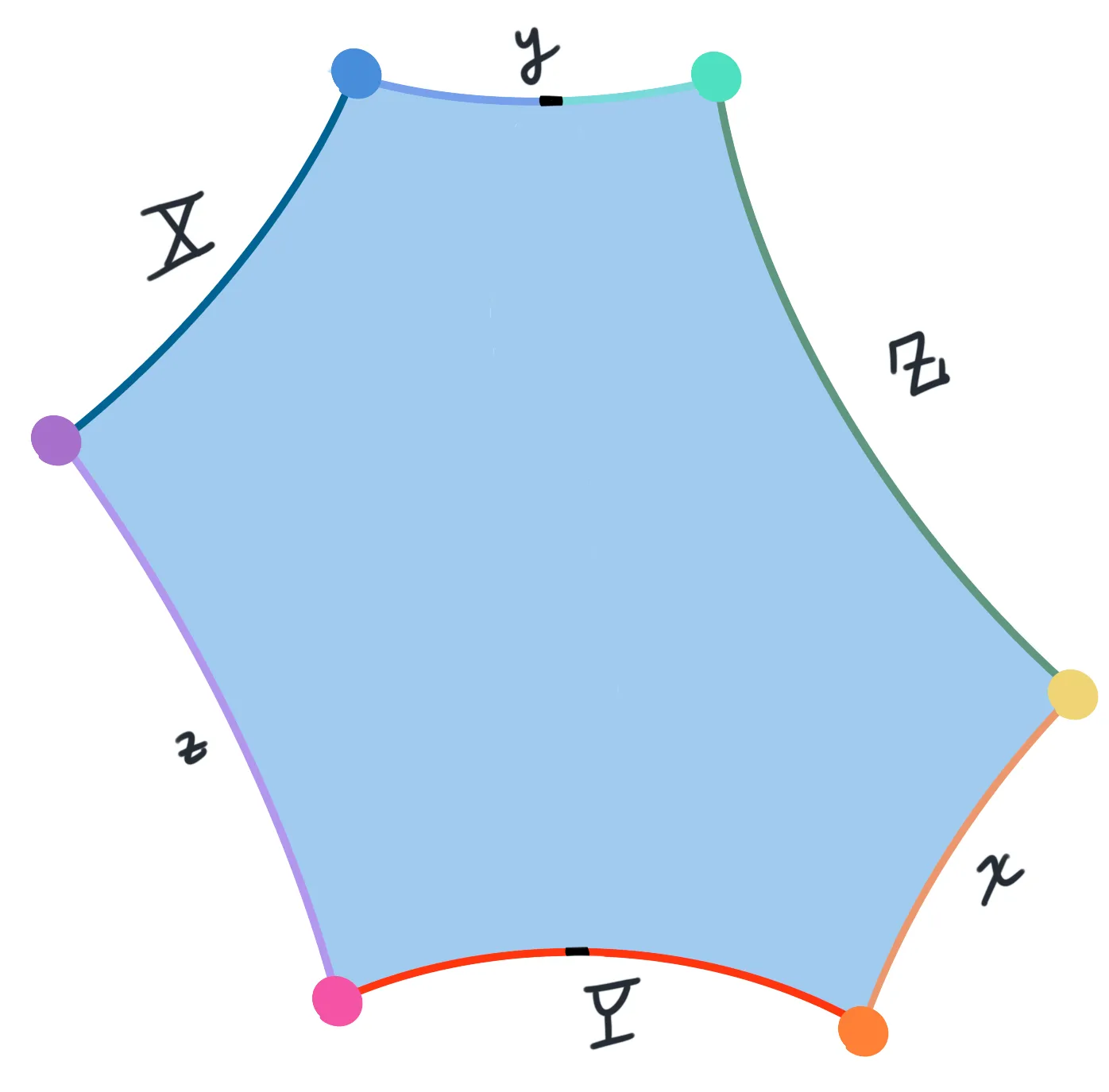
As we saw in Part I, there is a 3-dimensional moduli space of right angled hexagons in the plane, uniquely parameterized by specifying a triple of alternating side lengths.

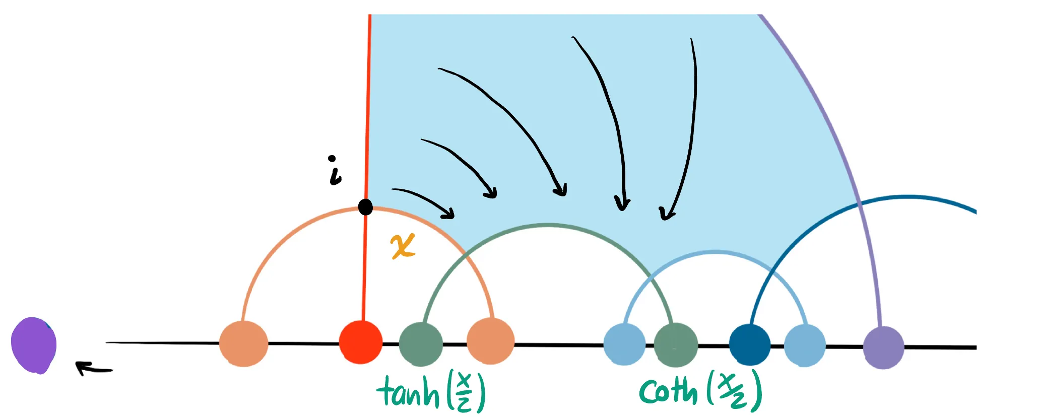
In this note, we compute a specific representation of such hexagons, by defining a map from such a triple to an ordered 6-tuple of geodesics. For concreteness we work in the upper half plane, where geodesics are faithfully represented by their endpoints, as an unordered pair in $\overline{\mathbb{R}}:=\mathbb{R}\cup\{\infty\}$. Such an explicit representation allows us to compute the group generated by reflections in the sides, and produce beautiful hyperbolic tilings as below:

PICTURE

It will be useful to recall a bit of notation: write the alternating known side lengths by $x,y,z$, and the three opposing sides as $X,Y,Z$ respectively. We will label each geodesic by its side length, so $\gamma_x$ represents the geodesic of side length $x$, and $\gamma_Z$ the geodesic of side length $Z$.

PICTURE

In Part I, we found the explicit formulas for $X,Y,Z$ in terms of $x,y,z$. Thus in our computations here we will freely use all six sides, knowing that three are already determined from the remainder.

$$\begin{align*} \cosh \left( X \right) &= \frac{\cosh(y) \cosh(z) + \cosh(x)}{\sinh(y) \sinh(z)} \\\\ \cosh \left( Y \right) &= \frac{\cosh(x) \cosh(z) + \cosh(y)}{\sinh(x) \sinh(z)}\\\\ \cosh \left( Z \right) &= \frac{\cosh(x) \cosh(y) + \cosh(z)}{\sinh(x) \sinh(y)} \end{align*}$$

Computing Geodesics in terms of Sides

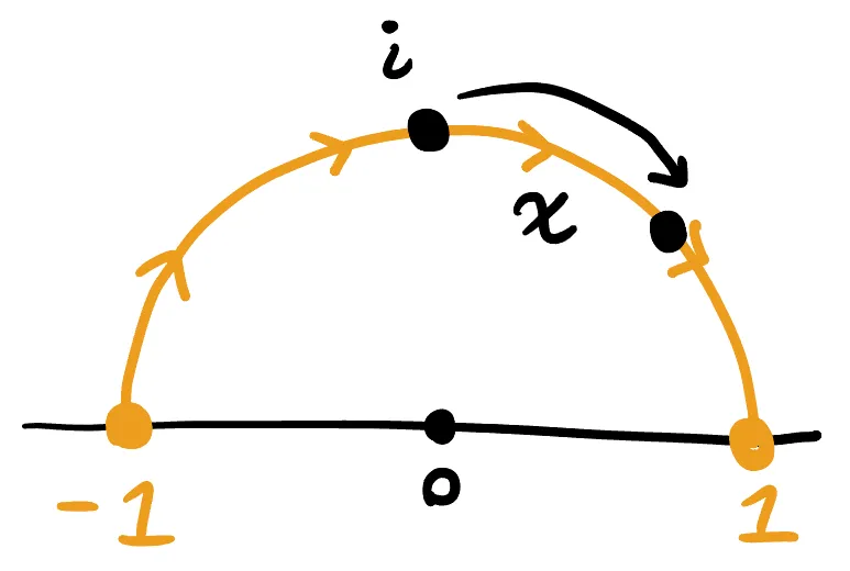
For each $(x,y,z)$ of side lengths we aim to compute one representative right angled hexagon, and so are free to use the isometries of the hyperbolic plane to simplify the problem. Indeed, using homogenity we can take one vertex $v$ of the hexagon to $i$, and then use isotropy to rotate it so one of the sides through $i$ is the unit circle. If we take this to be the side $x$, then

$\gamma_x \mapsto \{0,\infty\}$

But, as $H$ is right angled, the other side through $v=i$ must be perpendicular to the vertical - and thus, is the unit circle. This determines a second geodesic side:

$\gamma_Y\mapsto \{-1,1\}$

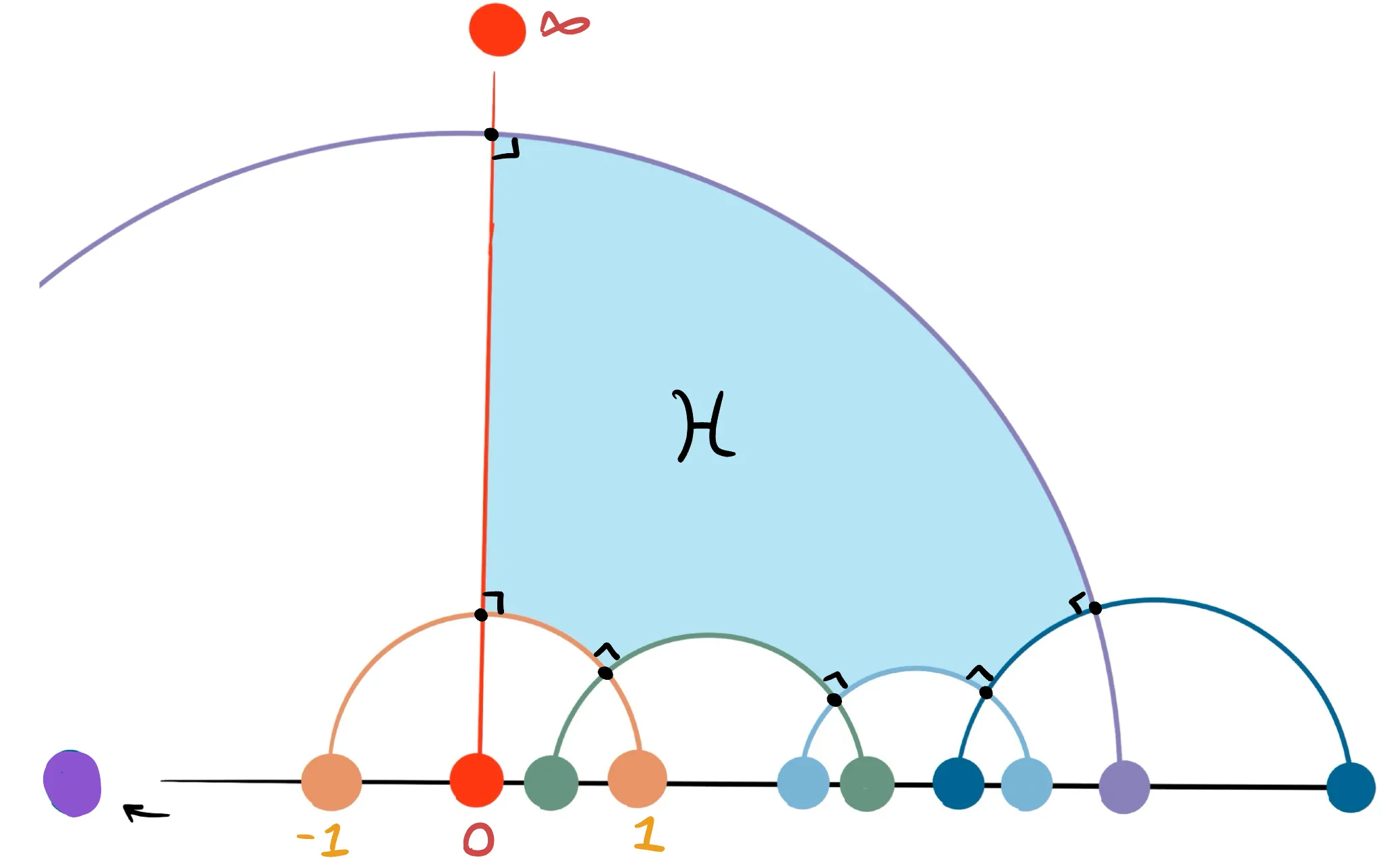
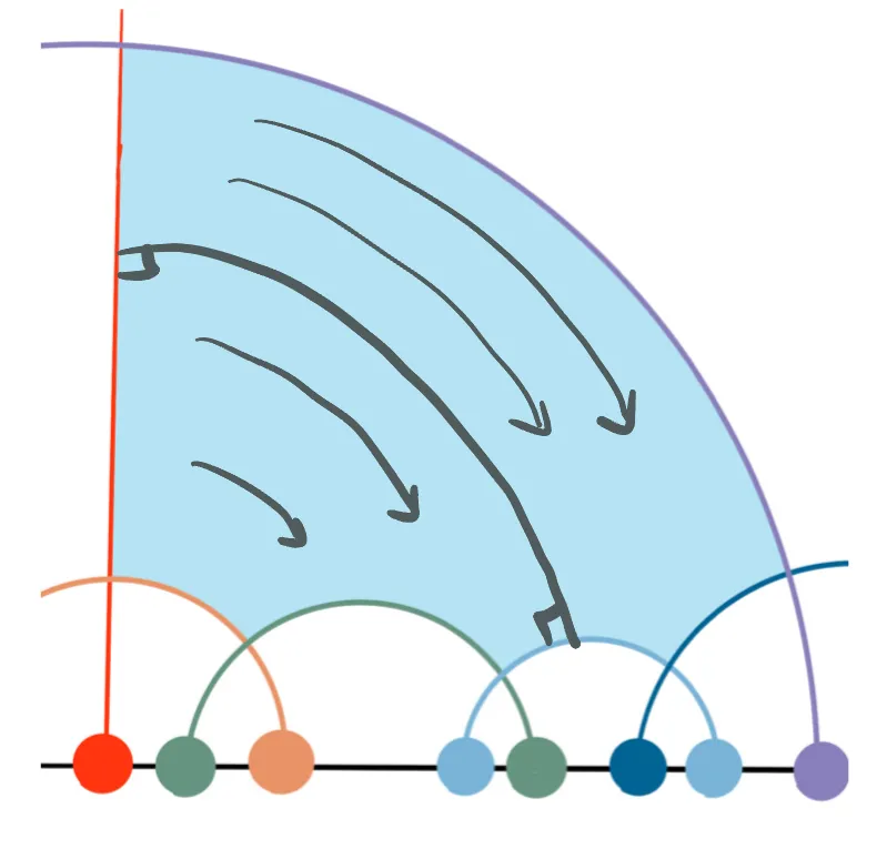
We have now fully used up the symmetry inherent to the problem, and will need to proceed to calculate the remaining four sides. We will later determine the lengths $X,Y,Z$ in terms of $x,y,z$; but for now we will work to express the endpoints of the remaining four geodesic sides in terms of these six quantities. The simplest of these to determine is the endpoints of the purple geodesic. Since it intersects the red (vertical) geodesic at a right angle, it must be a circle centered at the origin.

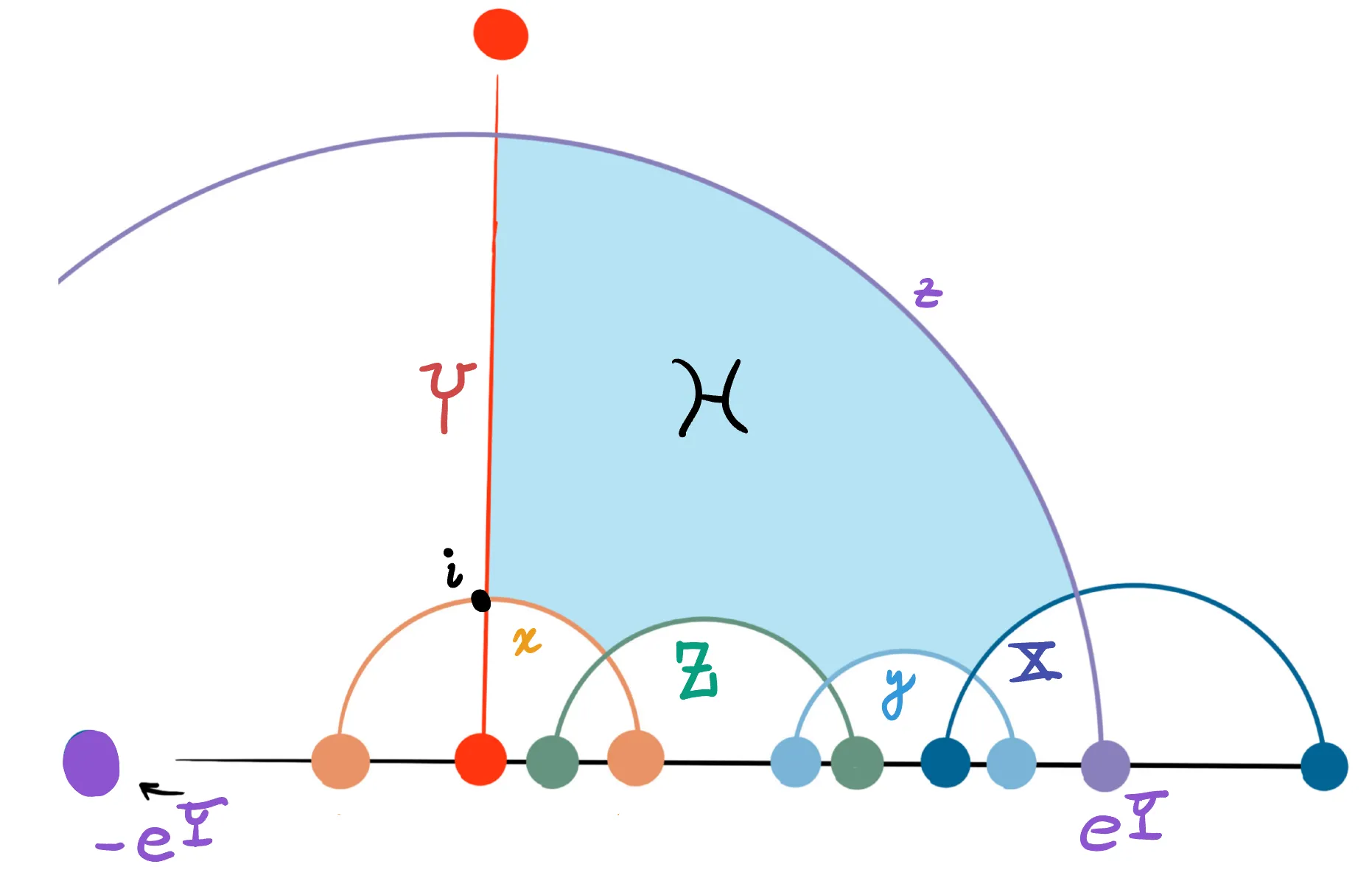
As the hyperbolic length of the vertical side is $Y$ and its first endpoint is at $i$, the second endpoint must lie at $e^Y i$ as

$$\begin{align} Y&=\mathrm{length}(\gamma_Y)\\ &=\int_1^? \frac{dt}{t}\\ &=\ln|t|\Big|_1^?\\ &=\ln(?) \end{align}$$

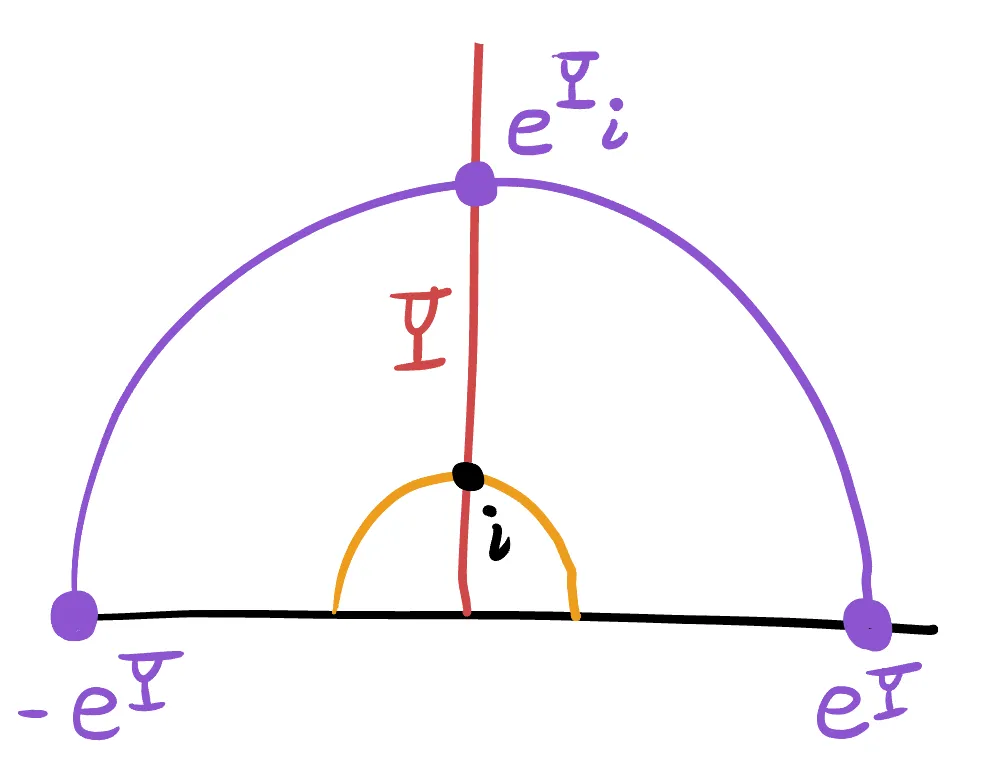
This fixes the geodesic of side length $z$: as the circle is centered at the origin and intersects the imaginary axis at $e^Yi$ it intersects the real axis at $\pm e^Y$.

$\gamma_z\mapsto \{-e^Y,e^Y\}$

Next, we proceed to calculate the endpoints of the green geodesic $\gamma_Z$:

Note that the hyperbolic isometry translating along the yellow edge $\gamma_x$ by distance $x$ takes the red-yellow intersection point to the yellow-green intersection point, and as both angles are right angles, necessarily takes the red geodesic to the green geodesic. Thus, the endpoints of the green geodesic are the images of $\{0, \infty \}$ under this isometry.

Translation by distance $x$ along the unit circle geodesic is accomplished by the Mobius transformation

$T=\begin{pmatrix}\cosh\frac{x}{2}&\sinh\frac{x}{2}\\\sinh\frac{x}{2}&\cosh\frac{x}{2}\end{pmatrix}$

Applying this to the endpoints $\{0,\infty\}$ of the red geodesic $\gamma_Y$ yields

$$\begin{align*} T_{0} &= \begin{pmatrix} \cosh \left( \frac{x}{2} \right) & \sinh \left( \frac{x}{2} \right) \\ \sinh \left( \frac{x}{2} \right) & \cosh \left( \frac{x}{2} \right) \end{pmatrix} \begin{pmatrix} 0 \\ 1 \end{pmatrix} = \begin{pmatrix} \sinh \left( \frac{x}{2} \right) \\ \cosh \left( \frac{x}{2} \right) \end{pmatrix} \rightarrow \tanh \left( \frac{x}{2} \right) \\ T_{\infty} &= \begin{pmatrix} \cosh \left( \frac{x}{2} \right) & \sinh \left( \frac{x}{2} \right) \\ \sinh \left( \frac{x}{2} \right) & \cosh \left( \frac{x}{2} \right) \end{pmatrix} \begin{pmatrix} 1 \\ 0 \end{pmatrix} = \begin{pmatrix} \cosh \left( \frac{x}{2} \right) \\ \sinh \left( \frac{x}{2} \right) \end{pmatrix} \rightarrow \coth \left( \frac{x}{2} \right) \end{align*}$$

Thus we have it;

$\gamma_Z\mapsto \left\{\tanh\frac{x}{2},\coth\frac{x}{2}\right\}$

We may calculate the endpoints of the indigo geodesic $\gamma_X$ similarly, by noting that it is the image of the red geodesic $\gamma_Y$ under translation along the purple edge $\gamma_z$ by a distance of z.

Because this purple edge is a circle centered at the origin, it is the image of the unit circle under translation along the vertical geodesic by $Y$. Thus, translation along the purple is given by conjugating translation along the unit circle by vertical translation. Precisely, let $V_Y\colon p\mapsto e^Yp$ be the translation of length $Y$ along the vertical geodesic, and $H_z$ be the translation by distance $z$ along the horizontal unit circle geodesic. Then the Mobius transformation $M$ we seek is

$M = V_YH_zV_Y^{-1}$

We are interested in the image of the red geodesic $\gamma_Y$‘s endpoints under this isometry. As $V_Y$ is translation along the red geodesic, it (and hence it’s inverse as well) fixes these endpoints, so

$$\begin{align} M.\{0,\infty\}&=V_YH_zV_Y^{-1}.\{0,\infty\}\\ &= V_YH_z \{0,\infty\} \end{align}$$

Using what we’ve previously learned about translation of $\{0,\infty\}$ along the unit circle, we see

$$\begin{align} V_YH_z.\{0,\infty\} &= V_Y.\left\{\tanh \frac{z}{2},\coth\frac{z}{2}\right\}\\ &=\left\{e^Y\tanh \frac{z}{2}, e^Y\coth\frac{z}{2}\right\} \end{align}$$

Thus we have it,

$\gamma_X \mapsto \left\{e^Y\tanh \frac{z}{2}, e^Y\coth\frac{z}{2}\right\}$

This leaves only the sky-blue geodesic $\gamma_y$ left to compute. There are two nice things we can try here: (1) we already know the green and indigo geodesics, and the blue geodesic is their common perpendicular. So we could use Euclidean geometry to find the unique circle centered on the real axis which is perpendicular to both of these circles. Or (2), we can continue with a method analogous to the above, and realize the blue geodesic as the image of the red (vertical) geodesic under some hyperbolic isometry.

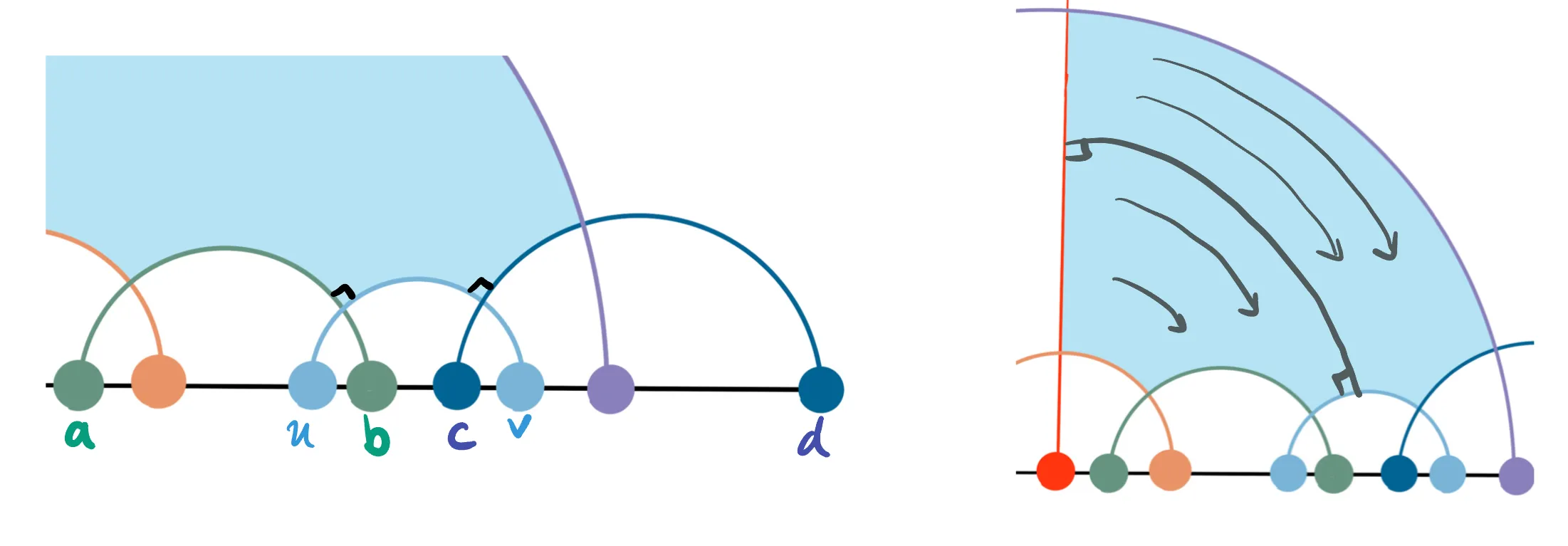
The second is considerably less messy in the end, so we proceed with (2). As the red and blue geodesics do not intersect, they have a common perpendicular, and, being perpendicular to the red geodesic, this is a circle centered at $o$. Say this common perpendicular intersects the red geodesic at a distance h from the red- yellow vertex, and is of length $d$.

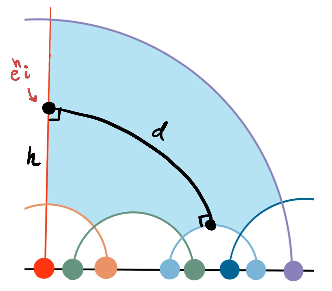
Precisely analogous to the previous case, we can realize translation along this common perpendicular as a conjugate of translation along the unit circle of distance $d$ by a translation along the vertical geodesic of distance $h$. This combination sends $\{0, A\}$ to the points

$\left\{e^h\tanh\frac{d}{2},e^h\coth\frac{d}{2}\right\}$

As written this formula is not exactly what we want: we wish to express everythign in terms of only $x,y,z$ and $X,Y,Z$; but this quantity involves the geometrically defined quantities $d$ and $h$ as well. To finish, we need to relate these to the side lengths. Doing so requires that we recall one important relation from the trigonometry of hyperbolic pentagons:

$\cosh(D)=\sinh(A)\sinh(B)$

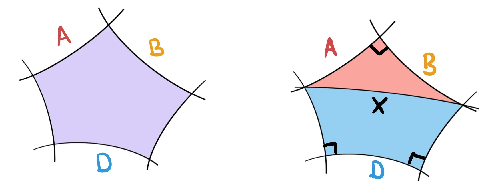
This is useful to us, as the common perpendicular of length $d$ divides the right angled hexagon $H$ into TWO right angled pentagons. We focus on the bottom pentagon, where we have labeled the side lengths (using * for the final side length, which proves irrelevant to our calculation).

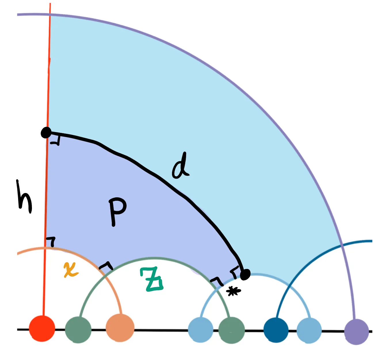
A right angled hyperbolic pentagon is determined up to isometry by any pair of adjacent side lengths, so the lengths $x,Z$ fully determine the remaining sides. Using these, we may then calculate the values of $h, d$ using the trigonometry of right angled hyperbolic pentagons, and the pair of adjacent sides $x,Z$.

$$\begin{align*} \cosh(d) &= \sinh(x) \sinh(Z) \\ \cosh(Z) &= \sinh(h) \sinh(d) \end{align*}$$

The first equation uniquely specifies a positive solution for $d$, and similarly the second implicitly determines a unique value of $h$. Thus, we are done and

$$\begin{align} \gamma_x &\mapsto \left\{e^h\tanh\frac{d}{2},e^h\coth\frac{d}{2}\right\}\\ d&=\operatorname{acosh}\left(\sinh(x)\sinh(Z)\right)\\ h&=\operatorname{asinh}\left(\frac{\cosh Z}{\sinh d}\right)\end{align}$$

Summary

Given the lengths $x,y,z,X,Y,Z$ we have found an explicit right angled pentagon $H$ having these as its side lengths, bounded by the geodesics

$\{0,\infty\},\{-1,1\},\{-e^Y,e^Y\}$ $\left\{\tanh\frac{x}{2},\coth\frac{x}{2}\right\}, \left\{e^Y\tanh\frac{z}{2},e^Y\coth\frac{z}{2}\right\}$ $\left\{e^h\tanh\frac{d}{2},e^h\coth\frac{d}{2}\right\}$ $d=\operatorname{acosh}\left(\sinh(x)\sinh(Z)\right)\hspace{0.25cm}h=\operatorname{asinh}\left(\frac{\cosh Z}{\sinh d}\right)$

In Code

Finally, here’s an actual implementation of this math, in the shader language GLSL, which I use to draw tilings such as at the top of this post.

//a geodesic is encoded by remembering its two boundary points
//these are real numbers (or the constant infty)
struct Geodesic{
    float p;
    float q;
};

//a  right angled hexagon is bounded by six geodesics
//we will call these a, b, c, d, e and f.
struct Hexagon{
    Geodesic a;
    Geodesic b;
    Geodesic c;
    Geodesic d;
    Geodesic e;
    Geodesic f;
};

Hexagon createHexagon(float x, float y, float z){

    Geodesic a,b,c,d,e,f;

    //sinh and cosh of the original side lengths
    float cx = cosh(x);
    float cy = cosh(y);
    float cz = cosh(z);

    float sx = sinh(x);
    float sy = sinh(y);
    float sz = sinh(z);

    //compute the opposing side lengths
    float cX = (cx+cy*cz)/(sy*sz);
    float cY = (cy+cx*cz)/(sx*sz);
    float cZ = (cz+cx*cy)/(sx*sy);

    float X = acosh(cX);
    float Y = acosh(cY);
    float Z = acosh(cZ);

    float sX = sinh(X);
    float sY = sinh(Y);
    float sZ = sinh(Z);


    //start computing the edges:

    //to the right of the vertical line
    a = Geodesic(0.,infty);

    //above the unit circle
    b = Geodesic(-1.,1.);

    //below the circle at height Y above unit circle
    f = Geodesic(exp(Y),-exp(Y));

    //above the circle which is translate of vertical line along unit circle by dist x
    c = Geodesic(tanh(x/2.),1./tanh(x/2.)),1.;

    //above the circle that is a translate by z along unit circle, then by Y along vertical geodesic
    e = Geodesic(exp(Y)*tanh(z/2.),exp(Y)/tanh(z/2.));

    //the final circle is the minimizing geodesic between the sides c and e:
    //this side is the image of the vertical line after translating D along unit circle, then h along vertical geodesic
    float cD = sx*sZ;
    float D = acosh(cD);
    float sD = sinh(D);

    float sh = cZ/sD;
    float h = asinh(sh);

    //the geodesic
    d = Geodesic(exp(h)*tanh(D/2.),exp(h)/tanh(D/2.));

    //finally we have the complete hexagon
    Hexagon H = Hexagon(a,b,c,d,e,f);
    return H;
}