Gauss' Linking Number I

Capturing the notion of linking in topology

\newcommand{\kl}{\widehat{K\text{-}L}}

Carl Friedrich Gauss was an alien. Or at least, sometimes it feels that way when I read his writings.

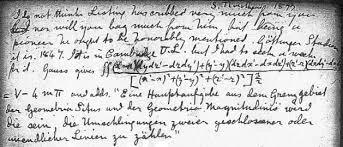
I recently came across Gauss’ first mention of what we now call the linking number of two smooth closed curves in $\mathbb{R}^3$. It appears almost offhandedly in his notebook, accompanied by a striking double integral—full of cross products and denominators—which somehow evaluates to an integer measuring how two curves are intertwined.

I vaguely remembered seeing this formula before, but I had never really thought carefully about where it comes from. I am not a knot theorist by training, and whenever I see a complicated formula that seems both canonical and mysterious, my instinct is that there must be a simpler conceptual story hiding underneath.

This post is the first in a short sequence working toward Gauss’ formula from first principles. The goal here is not to compute anything, but to understand what linking is actually measuring, and why it should give rise to an integer in the first place.

The question

Let $M^m$ and $N^n$ be two closed smooth manifolds embedded disjointly in $\mathbb{R}^{m+n+1}$. Typical examples to keep in mind are:

• a point and a curve in $\mathbb{R}^2$,
• two closed curves in $\mathbb{R}^3$,
• a curve and a surface in $\mathbb{R}^4$.

We would like to answer a deceptively simple question:

Are $M$ and $N$ linked?

At first glance this is hard to formalize. The embeddings contain a huge amount of information—exact shapes, parametrizations, curvature—most of which has nothing to do with linking. If we wiggle either manifold slightly without creating intersections, we do not expect the answer to change.

So the first task is not to compute anything, but to decide what information we should ignore.

How much information should we throw away?

A natural first thought is to consider embeddings up to isotopy: a continuous family of embeddings deforming one configuration into another. But isotopy remembers far too much. It keeps track not only of whether $M$ and $N$ are linked, but also of many fine details of how each manifold sits in space individually.

At the opposite extreme, we might try to work up to arbitrary homotopy. But this allows $M$ and $N$ to pass through one another, destroying exactly the phenomenon we are trying to capture.

What we really want is something in between. We want to forget how $M$ and $N$ interact with themselves, but still remember how they interact with each other.

Concretely, we will allow homotopies in which $M$ and $N$ are permitted to self-intersect—a single curve can pass through itself, like a loop of string pulled through its own body—but we insist that throughout the deformation the two manifolds remain disjoint from one another. This equivalence relation is known as link-homotopy, introduced by Milnor in the 1950s.

This is a deliberately coarse choice. It fails to distinguish certain links that isotopy can tell apart—for example, the Whitehead link is link-homotopically trivial despite being nontrivially linked. Detecting such subtleties requires more refined invariants (Milnor’s $\bar{\mu}$-invariants, for instance). But this coarseness is a feature, not a bug: Gauss’ invariant captures exactly this level of information—and no more.

Encoding disjointness using homotopy theory

The condition ”$M$ and $N$ remain disjoint” is awkward to express directly. The key trick is to package the data into a single map.

Given embeddings

$$K\colon M\to\mathbb{R}^p, \qquad L\colon N\to\mathbb{R}^p,$$

consider their product

$$K\times L\colon M\times N\to\mathbb{R}^p\times\mathbb{R}^p.$$

If $K$ and $L$ are disjoint, then $K(s)\neq L(t)$ for all $(s,t)$, so the image avoids the diagonal

$$\Delta=\{(x,x)\}.$$

Thus disjoint embeddings correspond to maps

$$M\times N\to\mathbb{R}^p\times\mathbb{R}^p\setminus\Delta.$$

Rather than track only those homotopies arising from product maps, we deliberately enlarge our equivalence relation and work with all homotopies into the complement of the diagonal. This can only make the invariant coarser: if the linking number detects something in this broader sense, it certainly detects it in the original sense. The payoff is that the problem is now squarely in the realm of homotopy theory.

Simplifying the target space

A simple change of coordinates gives homotopy equivalences

$$\mathbb{R}^p\times\mathbb{R}^p\setminus\Delta \;\simeq\; \mathbb{R}^p\setminus\{0\} \;\simeq\; S^{p-1},$$

where the first is induced by $(u,v)\mapsto u-v$ (the fiber over each nonzero point is a copy of $\mathbb{R}^p$, which is contractible) and the second is radial projection $x\mapsto x/\|x\|$.

So the linking data of $K$ and $L$ is encoded by a homotopy class of maps

$$[M\times N,\,S^{p-1}].$$

Under this identification, the product map becomes the normalized difference map

$$\kl(s,t)=\frac{K(s)-L(t)}{\|K(s)-L(t)\|}.$$

This map has a beautiful geometric interpretation: for each pair of points $s\in M$ and $t\in N$, it records the direction in space from $L(t)$ to $K(s)$. The linking question is now: as $(s,t)$ ranges over all of $M\times N$, does this collection of directions sweep out the sphere in a topologically essential way?

Linking is picky about dimension

A striking fact now emerges:

Linking is almost always trivial.

The only interesting case occurs when

$$p=m+n+1.$$

In smaller ambient dimensions, generic embeddings of $M^m$ and $N^n$ must intersect (there is not enough room to avoid one another), so the problem is better understood in terms of intersection theory. In larger dimensions, there is too much room: the product $M\times N$ has dimension $m+n$, and any map from an $(m+n)$-dimensional manifold into a sphere $S^{p-1}$ with $p-1>m+n$ can be contracted to a point. The intuition is dimensional: a low-dimensional domain cannot wrap around a higher-dimensional sphere, just as a curve in $\mathbb{R}^3$ cannot “surround” a $2$-sphere. More precisely, by cellular approximation the image can be deformed to miss at least one point of $S^{p-1}$, and the sphere minus a point is contractible.

Thus all nontrivial linking phenomena occur in a single “Goldilocks” dimension, where neither excess nor deficiency of ambient space prevents the map from being interesting.

Linking as a degree

In this special case, the normalized difference map

$$\kl\colon M\times N\to S^{m+n}$$

is a map between closed oriented manifolds of the same dimension $m+n$.

For maps between manifolds of the same dimension, there is a fundamental homotopy invariant: the degree. Intuitively, the degree of a smooth map $f\colon X^k\to Y^k$ between closed oriented $k$-manifolds counts, with sign, how many times $X$ “wraps around” $Y$ under $f$. One way to make this precise: pick a regular value $q\in Y$, and count the preimages $f^{-1}(q)$ with $+1$ if $f$ preserves orientation at that point and $-1$ if it reverses orientation. The sum is independent of the choice of regular value—this is the degree. A theorem of Hopf then shows that two maps $X\to Y$ are homotopic if and only if they have the same degree, so the degree is a complete invariant.

Applied to our setting: choose a direction $v\in S^{m+n}$, and ask for which pairs $(s,t)$ the direction from $L(t)$ to $K(s)$ is exactly $v$. The signed count of such pairs is independent of $v$—and this count is the linking number.

$$\operatorname{Link}(K,L):=\deg(\kl).$$

At this point we have achieved our first payoff: linking, defined via a fairly subtle equivalence relation on embeddings, reduces to a single integer.

In the next post, we will see how this abstract integer can actually be computed—converting the degree into an explicit integral using de Rham cohomology.