Sphere Linkages

Proving the configuration space of a chain suitably constrained at both ends is an n-sphere

Topology and geometry are full of wonderful, intricate, high-dimensional objects, but we are 3D creatures with 2D vision and getting any intuitive hold on a space of dimension $\geq 4$ is genuinely hard. But tere is a workaround I find delightful: high-dimensional spaces really are all around us — not embedded in physical space, but as the configuration spaces of physical things. The set of all possible arrangements of some mechanism is an abstract space, often a manifold, with its own topology and geometry, and we can interact with it tangibly by interacting with the mechanism.

The simplest examples come from rods and hinges. Pin one end of a rigid rod to the table and let the other swing free: the configuration space is a circle, $S^1$. Chain a second rod onto the end of the first, and each rod’s angle is independent — the configuration space is $S^1 \times S^1 = T^2$. Keep going, and a chain of $n$ rods with one end pinned has configuration space $T^n$, the $n$-torus — literally a product of $n$ circles handed to you on a plate. This might be the easiest way to put a high-dimensional space in your hands.

This series is part of an ongoing collaboration with Edmund Harriss, Aaron Abrams, and Dave Bachmann, where we’ve been thinking about how various corners of topology and geometry become tangible through configuration spaces of physical mechanisms. These blog posts are mostly me organizing my own thoughts as we go — notes from an ongoing exploration, not a polished writeup of a finished result.

In particular here we will take a narrow focus and think about the next simplest set of linkages after the n-torus: a chaing of n rods, held down not at one end, but two.

The tied-down-chain problem is rich, and its configuration space changes topology dramatically as the base length varies. The current set of three posts zooms in on a particular regime — base lengths close to fully stretched — where the configuration space turns out, surprisingly cleanly, to be an $n$-sphere. This post sets up the problem and proves the sphere result, recognizing adding a rod as a topological suspension. The second turns that suspension argument into a recipe for explicit spherical coordinates. The third equips these spheres with the kinetic-energy metric inherited from the underlying physics, and looks at the dynamics.

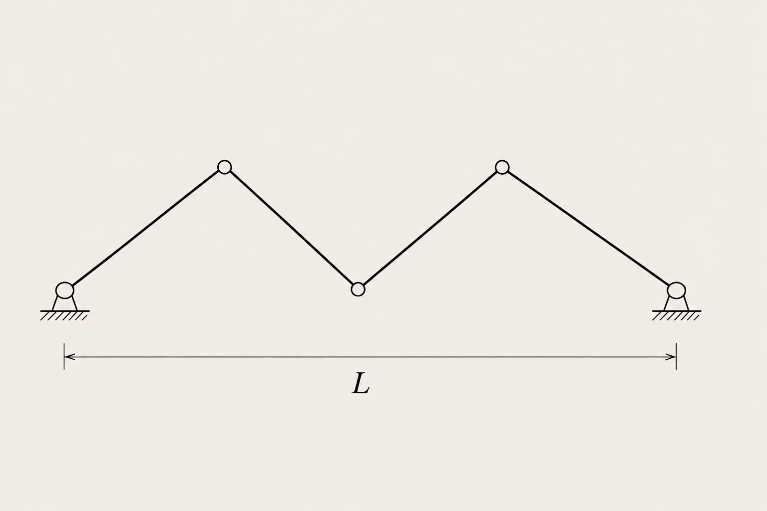
The setup

We work with a chain of $n$ unit rods hinged end-to-end in the plane, with both endpoints pinned a distance $L$ apart. Label the chain’s vertices $\mathbf{p}_0, \ldots, \mathbf{p}_n \in \mathbb{R}^2$, set $\mathbf{p}_0 := A = (0,0)$ by convention, and treat the remaining $n$ vertices as our variables. Two conditions govern them: each rod has unit length, $|\mathbf{p}_k - \mathbf{p}_{k-1}| = 1$ for $k = 1, \ldots, n$, and the chain is pinned at the far end, $\mathbf{p}_n = B := (L, 0)$. So our configuration space is:

$$\boxed{\; \mathcal{M}^n_L \;:=\; \left\{\; \begin{gathered} (\mathbf{p}_1, \ldots, \mathbf{p}_n) \in (\mathbb{R}^2)^n \;:\\ |\mathbf{p}_k - \mathbf{p}_{k-1}| = 1 \text{ for each } k, \\ \mathbf{p}_n = B \end{gathered} \;\right\}, \;}$$

with the convention $\mathbf{p}_0 := A$. This is an honest subset of $(\mathbb{R}^2)^n$, cut out by $n$ rigidity equations and $2$ endpoint-pinning equations. The ambient real dimension is $2n$, and there are $n + 2$ constraints — so if those constraints are everywhere independent, we’d expect $\mathcal{M}^n_L$ to have dimension $n - 2$.

Parameterizing by angles

We can cut the codimension down considerably by exploiting a fact we already know: each rod is a unit vector in the plane, which takes only one number to describe — its angle from the $x$-axis — not two. Building rigidity into the parameterization this way will leave only the closure condition to enforce.

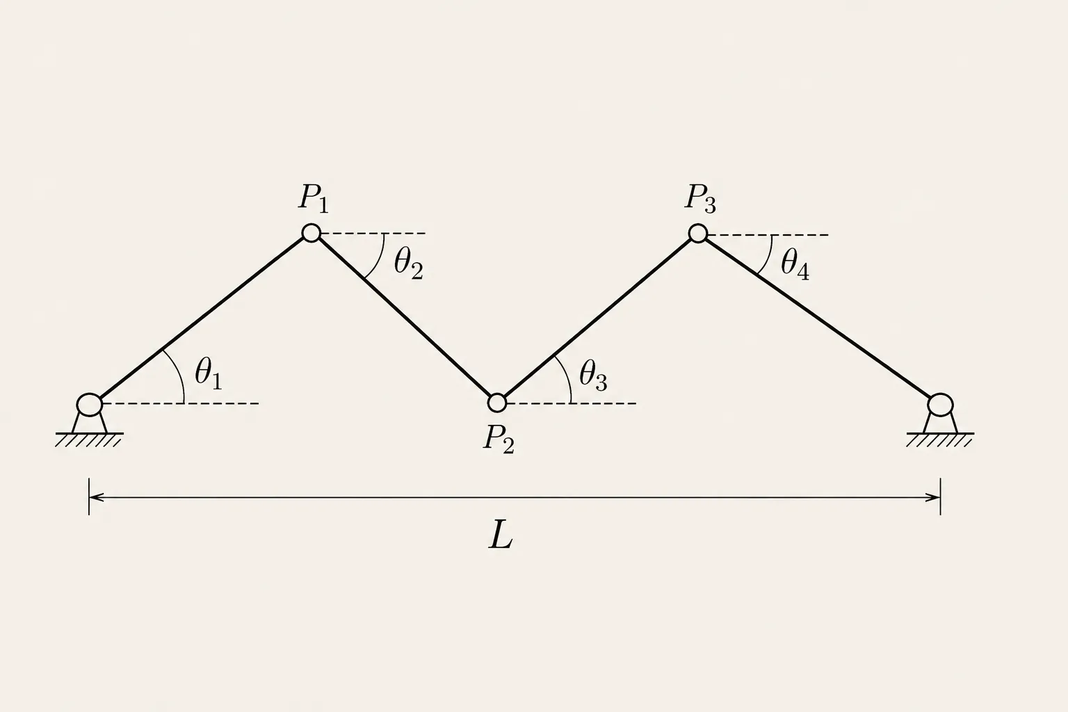
Identify $\mathbb{R}^2$ with $\mathbb{C}$. Given a tuple of angles $(\theta_1, \ldots, \theta_n) \in T^n$, build a chain by laying down the rods one at a time and recording the cumulative tip after each:

$$\begin{aligned} \Psi \;\colon\; T^n \;&\longrightarrow\; (\mathbb{R}^2)^n, \\ \Psi(\theta_1, \ldots, \theta_n) \;&=\; \big(\,e^{i\theta_1},\;\; e^{i\theta_1} + e^{i\theta_2},\;\; \ldots,\;\; \textstyle\sum_{j=1}^n e^{i\theta_j}\,\big). \end{aligned}$$

The $k$-th entry is the position of vertex $\mathbf{p}_k=\sum_{j=1}^k e^{i\theta_j}$ relative to $\mathbf{p}_0 = A$ at the origin. By construction $\mathbf{p}_k - \mathbf{p}_{k-1} = e^{i\theta_k}$, a unit vector, so $\Psi$ automatically lands in the rigid configurations — the rigidity constraints have been built in by the parameterization. The only remaining constraint, $\mathbf{p}_n = B$, transforms into a single complex equation in the angles:

$$\sum_{k=1}^n e^{i\theta_k} \;=\; L.$$

This is the closure equation. Pulling $\mathcal{M}^n_L$ back through $\Psi$ gives an alternative description as a codimension-2 subset of the $n$-torus,

$$\boxed{\; \mathcal{M}^n_L \;\cong\; \Big\{(\theta_1, \ldots, \theta_n) \in T^n \;:\; \textstyle\sum_k e^{i\theta_k} = L\Big\}, \;}$$

the level set of the complex-valued closure map $\Phi \colon T^n \to \mathbb{C}$, $(\theta_1, \ldots, \theta_n) \mapsto \sum_k e^{i\theta_k}$. A complex equation is two real equations, so $\mathcal{M}^n_L$ sits inside $T^n$ in codimension $2$ — a count consistent with the vertex picture’s expected dimension $n - 2$.

We can squeeze one more reduction out of the angle picture. Given the first $n - 1$ rod angles $(\theta_1, \ldots, \theta_{n-1})$, the position of vertex $\mathbf{p}_{n-1}$ is determined, and the last rod is forced: it has to point from $\mathbf{p}_{n-1}$ to $B$. The only remaining question is whether the required vector has unit length — that is, whether $|L - \sum_{k=1}^{n-1} e^{i\theta_k}| = 1$. When it does, $\theta_n$ is the argument of that vector and the configuration is closed. When it doesn’t, no value of $\theta_n$ rescues it.

So projecting onto the first $n-1$ angles gives an embedding $\mathcal{M}^n_L \hookrightarrow T^{n-1}$, cut out by a single real equation:

$$\boxed{\; \mathcal{M}^n_L \;\cong\; \Big\{\, (\theta_1, \ldots, \theta_{n-1}) \in T^{n-1} \;:\; \big|L - \textstyle\sum_{k=1}^{n-1} e^{i\theta_k}\big| = 1 \,\Big\}. \;}$$

Now we have a codim-1 subset of $T^{n-1}$ — same dimension $n - 2$ as before, but the ambient is one smaller, and the cutting equation is one real equation instead of two. We now have three descriptions of $\mathcal{M}^n_L$ and we’ll move freely between them. The first is the geometrically transparent vertex picture; the second is what makes the suspension structure visible (and proves the sphere theorem); the third is small enough that we can actually draw the configuration space for $n = 3, 4$, which we do next.

Experimentation

Before we prove anything about $\mathcal{M}^n_L$, we can actually look at it — the third description above is small enough to visualize for $n = 3, 4$ as we vary the base length $L$. Doing so will give us a feel for the space and, importantly, will tell us which range of $L$ to focus our analysis on.

$n = 3$. With three rods, $\mathcal{M}^3_L \subset T^2$ is the locus of $(\theta_1, \theta_2)$ where the third rod can close the chain — that is, where $|L - e^{i\theta_1} - e^{i\theta_2}| = 1$. Drawing the 2-torus as the square $[0, 2\pi]^2$ with periodic edges, $\mathcal{M}^3_L$ shows up as a curve.

Alternatively, we can wrap the periodic square back into the torus it represents and view $\mathcal{M}^3_L$ as a curve on the surface itself:

Sliding $L$ around, the curve does several different things. There’s a clear range where it looks like a single, cleanly-embedded loop on the torus — visibly a topological circle. Outside that range, the topology changes: the curve develops a self-crossing, splits into pieces, or disappears entirely.

$n = 4$. With four rods, $\mathcal{M}^4_L \subset T^3$ is a surface, the level set of $|L - e^{i\theta_1} - e^{i\theta_2} - e^{i\theta_3}| = 1$. Drawing the 3-torus as the cube $[0, 2\pi]^3$ with periodic faces, $\mathcal{M}^4_L$ becomes an isosurface.

Same story as $n = 3$. There’s a range of $L$ for which the surface looks unmistakably like a topological sphere — smooth, closed, unsplit. Outside that range it pinches, breaks into multiple components, or vanishes.

Reading off the regime. Eyeballing the experiments, the “nice” range looks like $1 < L < 3$ for $n = 3$ and $2 < L < 4$ for $n = 4$. The pattern is

$$n - 2 \;<\; L \;<\; n.$$

The upper bound $L < n$ is unsurprising: $n$ unit rods can’t span more than a distance of $n$, so beyond $L = n$ there are no configurations at all. The lower bound $L > n - 2$ is more interesting — it’s where the configuration space first stops being a sphere, and we’ll see in the next section that this corresponds to a degenerate “colinear” configuration becoming possible.

For the rest of this post we’ll work in this regime. The next section confirms what the experiments suggest — that $\mathcal{M}^n_L$ is a smooth manifold in this range — and the section after that proves it’s a sphere.

$\mathcal{M}^n_L$ is a smooth manifold

The experiments suggest a smooth manifold of dimension $n - 2$ throughout the regime $n - 2 < L < n$. But codimension counting alone doesn’t get us there — plenty of singular varieties are described as level sets — so we have actual work to do.

Theorem. For $n \geq 2$ and $n - 2 < L < n$, the configuration space $\mathcal{M}^n_L$ is a smooth submanifold of $T^n$ of dimension $n - 2$.

The standard tool for upgrading “level set” to “smooth submanifold” is the regular value theorem: if a smooth map $F \colon M \to N$ has $dF$ surjective at every point of $F^{-1}(y)$, then $F^{-1}(y)$ is a smooth submanifold of $M$ of codimension $\dim N$.

Notice that we have a choice of which description of $\mathcal{M}^n_L$ to plug in. Each of our three pictures presents it as a level set, and we can pick whichever makes the surjectivity check easiest:

1. Vertex picture. A level set in $(\mathbb{R}^2)^n$ cut out by $n + 2$ equations (rigidity plus endpoint pinning).
2. Codim 2 in $T^n$. A level set of the closure map $\Phi \colon T^n \to \mathbb{R}^2$, $(\theta_1, \ldots, \theta_n) \mapsto \sum_k e^{i\theta_k}$.
3. Codim 1 in $T^{n-1}$. A level set of $f \colon T^{n-1} \to \mathbb{R}$, $(\theta_1, \ldots, \theta_{n-1}) \mapsto \big|L - \sum_k e^{i\theta_k}\big|^2$.

Checking surjectivity onto a smaller codomain is generally easier — fewer rows of the Jacobian to worry about — so the vertex picture (codomain dimension $n + 2$) is by far the worst of the three. That leaves codim 2 and codim 1.

The codim-1 version has a 1D codomain, the simplest possible thing to be surjective onto. But when we write $f$ out in real coordinates,

$$f(\theta_1, \ldots, \theta_{n-1}) \;=\; \Big(\, L - \textstyle\sum_{k=1}^{n-1}\cos\theta_k \,\Big)^2 \;+\; \Big(\textstyle\sum_{k=1}^{n-1}\sin\theta_k\Big)^2,$$

the resulting partial derivatives are full of products and cross-terms. The codim-2 closure map, by contrast, has $\Phi$ equal to a single sum of trig functions in each component — its Jacobian, as we’ll see in a moment, is a clean $2 \times n$ matrix of sines and cosines that we can read information off by hand. Codim 2 is the sweet spot: a codomain small enough that surjectivity is easy to talk about, but a simple enough formula that the algebra actually goes through.

So we’ll work with $\Phi$. Identifying $\mathbb{C}$ with $\mathbb{R}^2$, the closure map’s real and imaginary parts give

$$\Phi \colon T^n \longrightarrow \mathbb{R}^2, \qquad \Phi(\theta_1, \ldots, \theta_n) \;=\; \Big(\, \sum_{k=1}^n \cos\theta_k,\;\; \sum_{k=1}^n \sin\theta_k \,\Big).$$

Its Jacobian — a $2 \times n$ matrix — is

$$D\Phi(\theta) \;=\; \begin{pmatrix} -\sin\theta_1 & -\sin\theta_2 & \cdots & -\sin\theta_n \\ \phantom{-}\cos\theta_1 & \phantom{-}\cos\theta_2 & \cdots & \phantom{-}\cos\theta_n \end{pmatrix}.$$

The $k$-th column is the unit vector $(-\sin\theta_k, \cos\theta_k) \in \mathbb{R}^2$.

For $D\Phi$ to be surjective onto $\mathbb{R}^2$, its image must span the plane — and that happens as soon as at least two columns are linearly independent. Equivalently, $D\Phi$ fails to be surjective only when every column is a scalar multiple of every other.

So we need to identify the configurations where this happens. Each column is a unit vector in $\mathbb{R}^2$, so for one to be a scalar multiple of another the multiplier has to be $\pm 1$ — the two columns are either equal or negatives of each other. Both cases mean the angles $\theta_j$ and $\theta_k$ differ by an integer multiple of $\pi$. So $D\Phi$ fails to be surjective exactly when all of $\theta_1, \ldots, \theta_n$ pairwise differ by multiples of $\pi$ — that is, when every rod points along a single common line.

What colinear configurations can satisfy closure? If all rods lie along a single common line, the chain itself — being the cumulative sum of the rod vectors — lies along that line too. Since the chain starts at the origin and ends at $(L, 0)$ with $L > 0$, the only candidate line is the positive $x$-axis. Each rod is therefore $\pm 1$, and the closure equation reduces to

$$L \;=\; n_+ - n_-,$$

where $n_\pm$ counts the rods pointing in the $\pm x$ direction — an integer. So $D\Phi$ can fail to be surjective only when $L$ is one of finitely many integer values, and for every other $L$ the regular value theorem immediately gives us a smooth manifold.

In our regime $n - 2 < L < n$ this rules out everything except a single point: $L = n - 1$, the lone integer in the interior. There the integer condition is met, and on the face of it a colinear configuration could exist. But the experiments showed nothing dramatic happening at $L = n - 1$ — the curve and surface looked perfectly smooth as we slid $L$ across that value — so we need to dig a little deeper.

The deeper observation is a quick parity calculation. We have two equations:

$$n_+ + n_- = n, \qquad n_+ - n_- = L,$$

the first because the rods partition into "$+$" and "$-$", the second from the colinear closure above. Adding them gives

$$2\, n_+ \;=\; n + L.$$

Since $n_+$ is a non-negative integer, the left side is even — so $n + L$ must be even too, which means $n$ and $L$ must have the same parity. The integer $L = n - 1$ has the opposite parity from $n$, so no integer $n_+$ can satisfy this equation. No colinear closure exists at $L = n - 1$: $D\Phi$ is surjective there too, and the regular value theorem applies.

Putting it together, $D\Phi$ is surjective at every point of $\mathcal{M}^n_L$ throughout the regime $n - 2 < L < n$, so $\mathcal{M}^n_L$ is a smooth submanifold of $T^n$ of dimension $n - 2$. This proves the theorem.

$\mathcal{M}^n_L$ is a sphere

We can now go further than smoothness:

Theorem. For $n \geq 2$ and $n - 2 < L < n$, $\mathcal{M}^n_L \;\cong\; S^{n-2}.$

The experiments already made $\mathcal{M}^4_L$ look like a $4-2=2$ sphere; the proof here formalizes this for every $n$. We argue by induction on the number of rods, with each inductive step recognizing the addition of a rod as a topological suspension. Starting from the base case $\mathcal{M}^2_L = S^0$ that gives a tower of $n - 2$ suspensions, and $\Sigma^{n-2} S^0 = S^{n-2}$ by repeated application of the formula below.

Definition (suspension). The (unreduced) suspension $\Sigma X$ of a space $X$ is the quotient of $X \times [0, 1]$ that collapses each end $X \times \{0\}$ and $X \times \{1\}$ to a single point. Picture latitudes of a sphere — each latitude a copy of $X$, the two poles the collapsed endpoints. In particular, $\Sigma S^k = S^{k+1}$.

We’ll keep the same coordinates as in the smooth manifold proof: $\mathcal{M}^n_L$ as the codim-2 subset of $T^n$, with all rod angles $\theta_1, \ldots, \theta_n$ explicit.

Base case: $\mathcal{M}^2_L \cong S^0$

Two unit rods from $A = (0,0)$ to $B = (L, 0)$, with $0 < L < 2$. The single interior hinge $\mathbf{p}_1$ lies on the unit circle around $A$ (because the first rod has length 1) and on the unit circle around $B$ (because the second rod has length 1). For $0 < L < 2$ those circles intersect in exactly two points,

$$\mathbf{p}_1^{\pm} \;=\; \left(\tfrac{L}{2},\; \pm \tfrac{\sqrt{4 - L^2}}{2}\right),$$

so $\mathcal{M}^2_L$ is a two-point space — i.e., $S^0$.

Inductive step: project onto the last rod

Assume inductively that $\mathcal{M}^{n-1}_d \cong S^{n-3}$ for every $d \in (n-3, n-1)$. We want to conclude $\mathcal{M}^n_L \cong S^{n-2}$ for $L \in (n-2, n)$.

Project a configuration onto the angle of its last rod:

$$\pi \colon \mathcal{M}^n_L \longrightarrow S^1, \qquad (\theta_1, \ldots, \theta_n) \longmapsto \theta_n.$$

(Either end of the chain would work topologically; we go with the last because peeling rods off the end leaves a sub-chain naturally indexed $(\theta_1, \ldots, \theta_{n-1})$ — ready to apply the same argument recursively, with no renaming.)

We’ll analyze the image and the fibers of $\pi$, and read the suspension structure off them.

Image of $\pi$. Given a last-rod angle $\theta_n$, the second-to-last vertex sits at

$$\mathbf{p}_{n-1} \;=\; B - e^{i\theta_n} \;=\; L - e^{i\theta_n}$$

— we just step backward from $B$ by one rod. The first $n - 1$ rods then need to span from $A$ to $\mathbf{p}_{n-1}$, which is possible iff $|\mathbf{p}_{n-1}| \leq n - 1$. So $\pi$ maps onto the arc

$$\theta_n \in [-\alpha, \alpha], \qquad \alpha \;=\; \arccos\!\left(\frac{L^2 - (n-1)^2 + 1}{2L}\right).$$

For $n - 2 < L < n$ this $\alpha$ lies strictly in $(0, \pi)$, so the image is a closed arc — topologically an interval, the suspension parameter we want.

Fibers of $\pi$. Fix $\theta_n$ in the admissible arc. The first $n - 1$ rods form a chain from $A$ to $\mathbf{p}_{n-1} = L - e^{i\theta_n}$, of sub-base length

$$d(\theta_n) \;=\; |L - e^{i\theta_n}| \;=\; \sqrt{L^2 - 2L\cos\theta_n + 1}.$$

In its own reference frame — with the base laid along the positive $x$-axis from $(0,0)$ to $(d, 0)$ — this sub-chain is a configuration in $\mathcal{M}^{n-1}_{d(\theta_n)}$. There is a unique orientation-preserving rigid motion identifying that sub-frame with the actual placement $A \to \mathbf{p}_{n-1}$, so the fiber

$$\pi^{-1}(\theta_n) \;\cong\; \mathcal{M}^{n-1}_{d(\theta_n)}.$$

By induction, what kind of fiber is this?

• Interior of the arc, $\theta_n \in (-\alpha, \alpha)$. A short calculation gives $L - 1 \leq d(\theta_n) < n - 1$, and since $L > n - 2$ we have $d > n - 3$. So $d$ stays strictly inside the inductive range, and the fiber is $\mathcal{M}^{n-1}_d \cong S^{n-3}$.
• Endpoints $\theta_n = \pm\alpha$. Here $d = n - 1$, the sub-chain is fully stretched, and $\mathcal{M}^{n-1}_{n-1}$ is a single point.

Putting these together, $\mathcal{M}^n_L$ is an arc’s worth of $(n-3)$-spheres, with each sphere collapsing to a single point at the two ends of the arc. That is precisely the unreduced suspension of $S^{n-3}$:

$$\mathcal{M}^n_L \;\cong\; \Sigma\, S^{n-3} \;\cong\; S^{n-2}. \qquad \blacksquare$$

What’s next

The suspension proof is short, but it is doing more work than just establishing the homeomorphism type. The argument is constructive: at each step it tells us how to coordinatize $\mathcal{M}^n_L$ using the suspension parameter $\theta_n$ together with whatever coordinates we already have on the fiber $\mathcal{M}^{n-1}_d$. Iterating from the base case $S^0$ all the way up — peeling off the last rod, then the next-to-last, and so on — gives explicit spherical coordinates on $\mathcal{M}^n_L$, with the full algebraic structure laid out as nested rotations and angles.

That recipe is the subject of the next post.